The Conviction Pyramid of Portfolio Construction
Hallerbach(2015): Advances in Portfolio Risk Control
Introduction
Ever since the birth of Mordern Portfolio Theory, mean variance optimization has taken a significant presence in portfolio construction, tilting the “science and art” blend a bit more toward the former. However, mean variance optimization is almost “notorious” for its sensitivity to small estimation errors in inputs, particularly when return and risk estimates are not well aligned.
It is especially the case during the dot-com and subprime crises when investors took the hard way to realize that parameter estimations are not as reliable as once thought. In facing of questions like “what if we cannot reliably forecast expected return, correlation, or volatility?”, risk-centric portfolio construction techniques that rely less on estimation, such as risk-weighted, risk parity, and maximum diversification, were created.
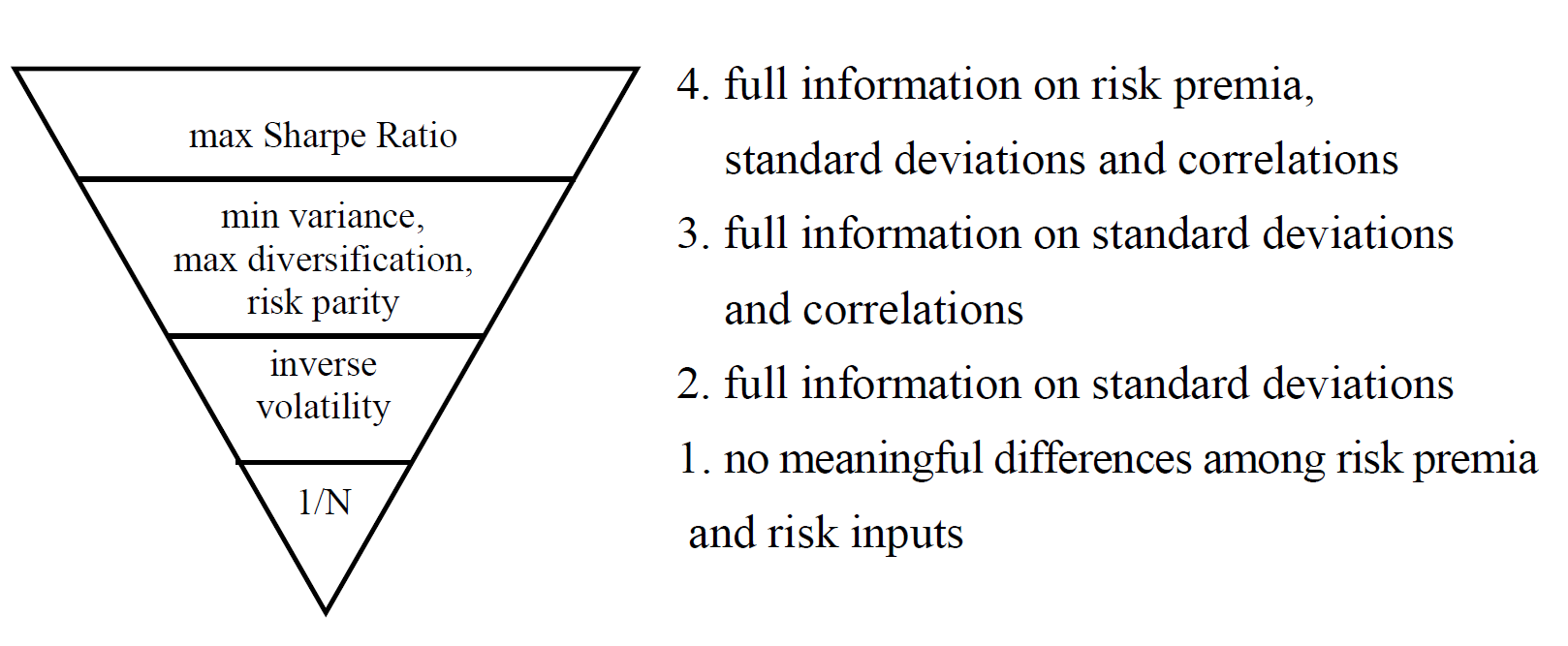
Hallerbach(2015) introduced a nice decision pyramid of portfolio construction, which links these portfolio construction methods with increasing input estimation requirements and difficulties. The pyramid starts from a scenario where nothing can be predicted reliably, up to a situation where both mean and variance are well understood.
The choice among these portfolio construction methods then depends on how confident we are in our forecasts. On one hand, the more reliable information we can feed into the portfolio construction process, the better performance we can expect from the portfolio. While on the other hand, poor estimation often have a detrimental negative impact on the portfolio.
In this blog post, I will try to delve into portfolio construction methods along Hallerbach’s decision pyramid. The objective is to gain some intuitive understanding of each method by examining their marginal conditions and aligning them with the mean variance efficient portfolio and each other.
Maximum Sharpe Ratio Portfolio
Let’s begin by setting the benchmark with the Maximum Sharpe Ratio Portfolio (MSRP). It is the tangent portfolio on the efficient frontier with highest sharpe ratio (\(\dfrac{R - R^{f}}{\sigma} = \dfrac{R^{e}}{\sigma}\)) across the opportunity set.
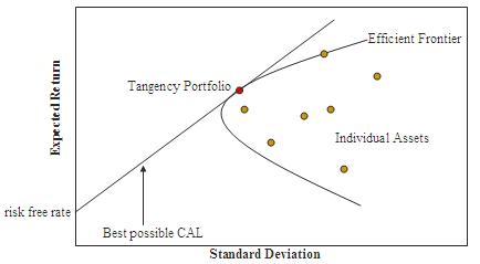
Source: wikipedia
The portfolio’s marginal condition offers nice insights. For a portfolio to be MSRP, the ratio of marginal contribution to excess return over marginal contribution to volatility from all constituents should align. Otherwise, one can improve the Sharpe ratio further by overweighting constituents with higher marginal ratios.
\[\begin{aligned} \dfrac{\partial R^{e}}{\partial w_i} / \dfrac{\partial \sigma}{\partial w_i} &= \dfrac{\partial R^{e}}{\partial w_j} / \dfrac{\partial \sigma}{\partial w_j} \\ \end{aligned}\]The marginal contribution to excess return of a constituent is simply its excess return. Thus we have
\[\begin{aligned} \dfrac{\partial R^{e}}{\partial w_i} &= r^{e}_i \\ \dfrac{1}{r^{e}_i} \dfrac{\partial \sigma}{\partial w_i} &= \dfrac{1}{r^{e}_j} \dfrac{\partial \sigma}{\partial w_j} \\ \end{aligned}\]It’s worth mentioning that, though not directly linked to a financial term, marginal contribution to volatility also plays a crucial role in portfolio analytics. It leads to an addible attribution of portfolio volatility to each constituent, with which one can decompose portfolio volatility to factor exposures, group of securities and so on. Qian (2006) further linked it to conditional percentile contribution of loss (under mild assumptions like normal distribution or 0 mean for short period), providing a nice financial interpretation for the quantity.
\[\begin{aligned} \sum_i w_i \dfrac{\partial \sigma}{\partial w_i} &= \sigma \end{aligned}\]Maximum Sharpe Ratio Portfolio (MSRP) is kind of the holy grail. In theory, it is the optimal portfolio for all investors, as it allows them to maximize expected returns for each unit of risk taken. Investors can adjust their leveage on MSRP to acheice a desired risk profile. However, accurate estimation of expected returns and the covariance matrix is crucial for achieving these results, and such estimations are not always readily available. When estimation errors occur, they can have a significant impact on the MSRP.
Without additional constraints, MSRP will consider our inputs as truth without any uncertainty and attempt to arbitrage with small differences within them, often unrealistically. For instance, if we estimate two securities with expected return of 10.5% and 10.7%, respectively, we do not want to place a heavy bet based on such a small difference. However, MSRP may view this as a serious arbitrage opportunity in case of high correlation. Such kind of unreasonable bets can result in a highly concentrated and unrealistic portfolio, which performs badly out of sample.
The sad fact remains that under quite some scenarios our estimations are no better than assertions like “all security share the same expected return”, “all asset classes share similar sharpe ratios”, “CAPM generally holds” …
Risk centric Portfolio Construction
That is when risk-centric portfolio can come into play. Risk-centric portfolio construction methods can help to address scenarios where reliable estimation is not available for certain inputs. Although these methods represent a compromise in the absence of reliable estimations, portfolios generated using them can be robust and perform comparably well to the true mean variance efficient portfolio in certain market scenarios (as suggested by their marginal conditions).
With no requirement for full knowledge on return and risk, these portfolio construction methods provide a conservative alternative with a solid bottom line and some upside potential for investors.
Equal Weight Portfolio (EWP) and Market Weight Portfolio (MWP)
At the bottom of the pyramid is the scenario neither return nor risk can be meaningfully differentiated. Hallerbach includes the equal-weighted portfolio (EWP) as a choice, which provides naive diversification based on money allocated. For sure it can deliver decent returns, while it also heavily loads on small-sized securities, leading to limited capacity and high transaction costs.
In practice, the market-weighted portfolio (MWP) is a more common choice (EWP as a backup for case that market value is not clearly defined. I.E derivative market). MWP is a very intersting portfolio with ascending information layers. For starter, it requires no input estimation and provides the portfolio with the largest capacity and lowest turnover based on the current market value. Additionally, if we are willing to take one step further with assumptions like homogenous expectation and all wealth in financial market. It is the MSRP portfolio as per CAPM.
For sure those are not assumptions hold all the time and CAPM is not an empirical success unconditionally. The MWP is still reasonably good in the sense that it is higly investibale with huge capacity. The relationship between expected return and market beta suggested by CAPM generally holds in an ambigous fashion. You might know about Warren Buffet’s famous bet with portfolio managers on wehter they could beat the market. The MWP is not easy to beat in practice. There is a whole industry of passive investing around market value weighted portfolios.
The fact that both EWP (DeMiguel, Garlappi & Uppal (2009)) and MWP are not easy to beat in practice also demonstrated the difficulty in accurately estimate inputs.
Risk Weighted Portfolio (RWP)
It is fortunate that volatility is usually much easier to estimate than other inputs with its consistent patterns of short-term clustering and long-term mean reversion. As we move up the portfolio pyramid to the case when estimation on volatility is available, we gain access to methods that can help us understand and manage risk better.
One such method is the Risk Weighted Portfolio (RWP), which goes beyond naive diversification in terms of money invested. Instead, it diversifies based on the volatility involved with securities’ weights inversely related to their volatility (I.E: \(w_i = \dfrac{\dfrac{1}{\sigma_i}}{\sum_j \dfrac{1}{\sigma_j}}\)). This approach leads to a more risk aware decision compared to the EWP and can help investors benefit from the well-known low-risk anomaly. Securities with low risk tend to have higher expected returns than originally expected due to rationales like institutional constraints. RWP implicitly help investors to exploit such market anomaly and lead to more efficient risk-taking.
Incorporating correlation estimation moves us higher up the portfolio pyramid and provides a relative comprehensive disclosure on the risk front. This in turn allows us to leverage a range of sophisticated methods, such as Mean Variance (MVP), risk parity portfolio (RPP), and Maximum diversification portfolio (MDP) to better manage risk and take advantage of the benefit in diversification. Each of these methods has its own unique philosophy and approach, and is justified based on the goals and preferences of the investor.
Minimum Variance Portfolio (MVP)
The Minimum Variance Portfolio (MVP) is a portfolio optimization method that seeks to minimize overall portfolio volatility. Like the RWP, MVP benefits from the low volatility anomaly. What sets MVP apart is that it is the only portfolio on the efficient frontier that does not depend on expected return estimation.
To construct a MVP, the marginal contribution to volatility must be equal for every security, which makes it equivalent to MSRP if every security share the same excess return. In general, MVP puts more weights on securities with smaller volatility and lower correlation to others.
\[\begin{aligned} \dfrac{\partial \sigma}{\partial w_i} &= \dfrac{\partial \sigma}{\partial w_j} \end{aligned}\]Risk Parity Portfolio (RPP)
Risk Parity Portfolio (RPP) is another popular choice that seeks to allocate risk equally among all constituents of a portfolio. It can be applied to risk metrics other than volatility, and can also consider other concepts like macroeconomic scenarios as constituents. The idea behind RPP is to create a diversified portfolio where every constituent contributes equally to the overall risk of the portfolio. This is achieved by setting the weight of each constituent proportional to its contribution to the total portfolio risk.
\[\begin{aligned} w_i \dfrac{\partial \sigma}{\partial w_i} &= w_j \dfrac{\partial \sigma}{\partial w_j} \end{aligned}\]When all constituents have the same ratio of excess return over its risk contribution, RPP becomes return risk efficient (MSRP), making it actually a good starting point for asset allocation. As from a long-run equilibrium perspective the ratio of return to systematic risk is expected to be relatively stable across different asset classes, avoiding arbitrages on one or some becoming dominant over others. Empirically RPP did perform well in the low-interest-rate environment of the last few decades. When coupled with leverage, RPP deliver reasonable return with a high sharpe ratio historically.
However, in its nature, RPP is sensitive to volatility (whether it originates from reality or estimation error). That will become a problem if gap in volatility between equity and fixed income is huge as RPP is overly concentrated in low risk assets. Take the Chinese financial market as an example, the historical realized volatility of equity and treasury are around 30% and 5% respectively. A typical RPP in the case would generally lead to a portfolio with more than 95% of weight in treasury, a extremly conservative portfolio that do not fit most investors’ objective.
The difference in volatility is much more balanced in the Developed Market. While still, RPP generally leads to a portfolio that comes with high sharpe ratio but low risk profile. It requires high leverage to achieve the desried level of risk and return. Those leverage can be hard to achieve or bring further risk and cost in marketing to market. There are quite some research calling into questions about the good historical performance of RPP from pespectives of interest rate environment, futhre information, cost and so on.
It’s also important to notice that, unlike MVP, RPP is sensitive to the definition of asset classes. It is completely different thing to conduct RPP among two classes of equity and fixed income or among a different grouping of DM equity, EM equity, fixed income and alternatives. While in practice, financial markets are grouped into different sub groups due to all kinds of business considerations hence not all asset classes should come with the same importantce. In that case risk budget that assign subjective proportion of risk to each asset class makes more sense.
\[\begin{aligned} \dfrac{w_i}{budget_i} \dfrac{\partial \sigma}{\partial w_i} &= \dfrac{w_j}{budget_j} \dfrac{\partial \sigma}{\partial w_j} \end{aligned}\]Maximum Diversification Portfolio (MDP)
Last but not least, we have the maximum diversification portfolio (MDP) that maximize the diversification ratio (\(\dfrac{\sum_i \sigma_i}{\sigma}\)). It is a direct implemention of the concept that “diversification is the only free lunch in finance”.
Taking its marginal condition, it is clear that MDP is equivalent to MSRP when the sharpe ratio of all constituents align, which is something can be expected every once a while.
\[\begin{aligned} \dfrac{1}{\sigma_i} \dfrac{\partial \sigma}{\partial w_i} &= \dfrac{1}{\sigma_j} \dfrac{\partial \sigma}{\partial w_j} \end{aligned}\]In my experience, what makes MDP particularly handy is the availability of multiple MDPs corresponding to different risk targets, which provides investors with flexibility in achieving a desired risk profile without relying heavily on leverage. MDP with risk targets is one reasonable implementation of the idea to determine the absolute risk level first, and then allocate it to each asset class in a way that maximizes diversification. It seems to be a solid reasoning when reliable return estimation is not available.
Furthermore, the marginal condition where each side of the equation is scaled by volatility reveals that correlation, rather than volatility, plays a more critical role in determining the MDP. This avoids the RPP scenario with large volatility gaps in constituents, but also makes the portfolio sensitive to changes in correlation, which for sure is not an invariant quantity.
Reference
- Hallerbach (2015): Advances in Portfolio Risk Control
- Qian (2006): On the Financial Interpretation of Risk Contribution: Risk Budgets do add up
- Choueifaty (2008): Torward maximum diversification
- Haesen, Hallerbach & Markwat (2017): Enhancing Risk Parity by Including Views
- DeMiguel, Garlappi & Uppal (2009): Optimal Versus Naive Diversification: How Inefficient is the 1/N Portfolio Strategy?