Nowcasting: The News From Jagged Economic Data
- Economic Indicators: the informative and nerve-wracking data flow
- The Nowcasting modeling of Economic Indicators
- EM Estimation
- The Practical Aspect
- Reference
Economic Indicators: the informative and nerve-wracking data flow
Financial market is like a bustling abstraction of the economic world, where people jump into the bus for economic objects such as sharing income and mitigating risk. Therefore, it comes as no surprise that economic conditions are quite relavant in participating in the market.
This notion finds its support in empirical research as well. Scholars and industry experts have dedicated considerable efforts to conduct studies, revealing the profound influence of various economic factors on the performance of asset classes, yield curves, sectors, styles, and so on. It hilighted the importance of considering economic conditions when making informed investment decisions.
However, it is not a straghtforward task to incorporate the data flow of economic indicators into a regular investment decision process. We are faced with an overwhelming number of economic indicators that are unstructured in their natures.
Economic Data Flow: Jagged and Mixed Frequency
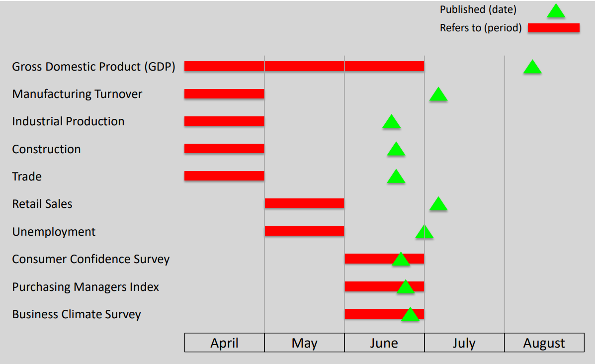
Lucrezia Reichlin’s Presentation on Nowcast
Just as the chart above glimpses, the complexity arises generally from two aspects. On one hand, these indicators are published at different frequencies. For example, GDP is published quarterly, PMI is published monthly, railroad traffic is published weekly… etc. On the other hand, the publish schedule can vary significantly for different indicators. For instance, GDP and Industrial Production are typically published less than two months after the reporting period, while PMI is usually published immediately after the reporting period. Let alone there are regular revise on economic indicators after its initial publish. Traditional econometrical method like OLS can’t deal with such jagged data efficiently!
Fortunately, we have the nowcasting model at our disposal to navigate this complex data flow. Originally developed with a primary focus on monitoring GDP growth at central banks, the nowcast model provides a cohesive statistical framework to handle the irregular and mixed-frequency nature of economic data flow. This model empowers us to establish a robust system that continually updates our insights on economies based on the incremental release of data, regardless of its irregular frequency and release schedule.
In this blog, we will explore the remarkable capabilities of the nowcasting model. We will delve into the intuition behind this powerful tool, focusing on its modeling and estimation aspects. Additionally, we will provide practical insights on ways to incorporate this model into the decision-making process through illustrative toy examples.
The Nowcasting modeling of Economic Indicators
Embarking on our exploration, let’s delve into the inner workings of the nowcasting model.
At its core, the nowcasting model is built on the foundation of a dynamic factor model (DFM). This powerful framework is further enhanced by incorporating equations that link economic indicators at different frequencies and leveraging a customized EM (Expectation-Maximization) algorithm. By doing so, the nowcasting model effectively tackles the challenges posed by mixed-frequency and irregular data flow. It treats indicators not yet published as missing values and handle them seamlessly via the Kalman filter, ensuring robust and up-to-date insights into economic conditions.
Dynamic Factor Model
As the foundation of a nowcast model, the DFM aims to find a concise set of latent factors that drive a significant portion of the variation across a wide array of observed economic indicators. What set the DFM apart as “dynamic” is that it jointly model and estimate both the observed economic indicators and the transition dynamics of the latent factors.
In the nowcasting model, all economic indicators are modeled at their highest frequency. The observed economic indicators, denoted as \(y_t\), are governed by a small set of latent factors, denoted as \(f_t\). Each latent factor represents a specific aspect of the economy.
A typical DFM representation of nocasting model is as follows. \(\Lambda\) is the loading matrix that determines how each economic indicator is driven by the latent factors and matrix \(A_p\) governs the evolution of the latent factors themselves. The dynamics of the latent factors and the idiosyncratic components \(\epsilon_t\) are captured via vector autoregressive process (VAR).
\[\begin{aligned} y_t &= \mu + \Lambda f_t + \epsilon_t \\ f_t &= A_1 f_{t-1} + ... + A_p f_{t-p} + u_t \\ \epsilon_{i,t} &= \alpha_i \epsilon_{i, t-1} + ... + e_{i,t} \\ u_t &\sim N(0, Q) \\ e_{i, t} &\sim N(0, I) \end{aligned}\]What’s worth metioning is that it’s also quite easy to impose further structures in the model. For instance, Banbura, Giannone & Reichlin(2010) partitioned the lattent factors into 3: One global factor \(f_t^{G}\) that loads on every economic indicator and summarize the general economic condition and two factors \(f_t^{N}, f_t^{R}\) that loads on nomial indicators and real indicators separately to account for cross section structure within real and nominal indicators.
Such a formation can be easily implemented by imposing restrictions on the loading matrix, the transition matrix, and the covariance matrix as below. The adoption of a customized EM algorithm (more detials later) ensures that such restriction does not pose much problem during estimation.
\[\Lambda = \begin{bmatrix} \Lambda_{N,G} & \Lambda_{N,N} & 0 \\ \Lambda_{R,G} & 0 & \Lambda_{R,R} \end{bmatrix}\] \[A_i = \begin{bmatrix} A_{i,G} & 0 & 0 \\ 0 & A_{i, N} & 0 \\ 0 & 0 & A_{i,R} \end{bmatrix}\] \[Q = \begin{bmatrix} Q_G & 0 & 0 \\ 0 & Q_N & 0 \\ 0 & 0 & Q_R \end{bmatrix}\]Handling of mixed frequency
Given that the model operates at the highest frequencies of all economic indicators, it is necessary to establish a link to handle and incorporate indicators published at lower frequencies. To illustrate, let’s consider the integration of GDP into a monthly model as an example.
Suppose \(GDP_t\) represents the unobservable monthly GDP amount. To integrate the observable QOQ GDP growth (\(x_t^{Q} = log(\dfrac{GDP_{t-2} + GDP_{t-1} + GDP_t}{GDP_{t-5} + GDP_{t-4} + GDP_{t-3}})\)), we need to align it to the unobserved MOM GDP growth (\(x_t^{M} = log(\dfrac{GDP_t}{GDP_{t-1}})\)) to ensure a meaninful comparison with other monthly indicators and then incorporate the quarterly series through the established link.
Mariano and Murasawa (2003) introduced the following linking function as one way to do the work.
\[\begin{aligned} log(\dfrac{GDP_{t-2} + GDP_{t-1} + GDP_t}{GDP_{t-5} + GDP_{t-4} + GDP_{t-3}}) &\approx log(\dfrac{GDP_t}{GDP_{t-1}} (\dfrac{GDP_t-1}{GDP_{t-2}})^2 (\dfrac{GDP_t-2}{GDP_{t-3}})^3 (\dfrac{GDP_t-3}{GDP_{t-4}})^2 \dfrac{GDP_4}{GDP_{t-5}}) \\ &= log(\dfrac{GDP_t * GDP_{t-1} * GDP_{t-2}}{GDP_{t-3} * GDP_{t-4} * GDP_{t-5}})\\ &\downarrow \\ x_t^{Q} &\approx x_{t}^M + 2x_{t-1}^M + 3x_{t-2}^M + 2x_{t-3}^M + x_{t-4}^M \end{aligned}\]Assuming the MOM GDP growth \(x_t^M\) follows the same factor model structure as other monthly indicators, we can model \(x_t^Q\) with lagged latent factors without messing around the relationship between QOQ growth and MOM growth.
\[\begin{aligned} x_t^M &= \mu_Q + \Lambda_Q f_t + \epsilon_t^Q \\ &\downarrow \\ x_t^Q &= 9 \mu_Q + \Lambda_Q f_{t} + 2\Lambda_Q f_{t-1} + \Lambda_Q f_{t-2} + \Lambda_Q f_{t-3} + \Lambda_Q f_{t-4} + \epsilon_{t}^Q + 2\epsilon_{t-1}^Q + 3\epsilon_{t-2}^Q + 2\epsilon_{t-3}^Q + \epsilon_{t-4}^Q \end{aligned}\]The following extended DFM can be used to incorporate the quarterly QOQ GDP growth. Still within the same DFM framework :)
\[\begin{bmatrix} y_t \\ x_t^Q \end{bmatrix} = \begin{bmatrix} \mu \\ \mu_Q \end{bmatrix} + \begin{bmatrix} \Lambda &0 &0 &0 &0 &I_n &0 &0 &0 &0 &0 \\ \Lambda_Q &2\Lambda_Q &3\Lambda_Q &2\Lambda_Q &\Lambda_Q &0 &1 &2 &3 &2 &1 \end{bmatrix} \begin{bmatrix} f_t \\ f_{t-1} \\ f_{t-2} \\ f_{t-3} \\ f_{t-4} \\ \epsilon_{t} \\ \epsilon_{t}^Q \\ \epsilon_{t-1}^Q \\ \epsilon_{t-2}^Q \\ \epsilon_{t-3}^Q \\ \epsilon_{t-4}^Q \\ \end{bmatrix}\]Similar tricks can be deduced easily to mimic other mixed-frequencies dynamics.
Handling of jagged publish
Incorporating data with mixed frequencies into the DFM is definitely a milestone for our quest, but there are still challenges to overcome. As in the GDP example, we have a model with all indicators intervaled at 1 month while GDP is published every three months. How can we haddle months when GDP release is not available?
This dilemma of uneven data availability arise not only with indicators at lower frequencies but also with indicators that are yet to be published. As mentioned earlier, economic indicators can have reporting delays ranging from 0 up to 60 days after the reporting period. While options remain to wait for all indicators to become available before resuming the modeling and estimation process or simply select indicators with short delays, these approaches comes at the significant cost of losing comprehensive up-to-date insights.
To address this challenge, nowcasting models make effective use of the Kalman filter in the estimation process. With Kalman filter used in the E step of EM algorithm, the nowcasting model can treat unpublished indicators as missing values and fills in the gaps with estimated conditional means during the initial estimations. \(\Omega_{t_i}\) below refers to all information published up to point \(t_i\)
\[\begin{aligned} & E(y_t | \Omega_{t_i}) & E(f_t | \Omega_{t_i}) \end{aligned}\]When the economic indicator eventually becomes available upon later publish, it can be seamlessly integrated into the existing nowcasting model through Kalman filter updates. This ensures that the model remains comprehensive and up-to-date, providing valuable insights into the current economic landscape. Other indicators remaining unpublished and lattent factor can be updated linearly on the increamental info. The incremental addtion of \(\Omega_{t_{i+1}}\) over \(\Omega_{t_i}\) can be publish of newest indicators as well as revise of historical indicators.
\[\begin{aligned} & E(y_t | \Omega_{t_{i+1}}) & E(f_t | \Omega_{t_{i+1}}) \end{aligned}\]EM estimation
With the utilization of linking functions and Kalman filters, we finally obtained a model that can effectively handle the jagged and mixed-frequency data. While before delving into the practical usage of the model, let’s take a detour and discuss the customized EM algorithm required for estimation. After all, a model can be as comprehensive and accurate as it can, but it is of little use if there is no reliable way to estimate the parameters.
For a regular (DFM) where all variables \(y_t\) are observed, an EM algorithm involving Kalman smoother and two multivariate regressions can be used for estimation. For each iteration of the algorithm:
In the E (Expectation) step the Kalman smoother is utilized to estimate the conditional moments of latent factors:
\[\begin{aligned} &E_j(f_t|\Omega_{t_i}) &E_j(f_t f_t^{'}|\Omega_{t_i}) \\ &E_j(f_{t-1} f_{t-1}^{'}|\Omega_{t_i}) &E_j(f_{t} f_{t-1}^{'}|\Omega_{t_i}) \end{aligned}\]Additionaly, the conditional moments of observed indicators can be estimated as follows:
\[\begin{aligned} E_j(y_t y_t^{'}|\Omega_{t_i}) &= y_t y_t^{'} \\ E_j(y_t f_t^{'}|\Omega_{t_i}) &= y_t E_j(f_t^{'}| \Omega_{t_i}) \end{aligned}\]In the M (Maximization) step two regressions are used to estimate the loading matrix and transition matrix respectively. Completing one iteration of the EM involves plugging in the conditional moments from the E step in the slope of both regressions.
\[\begin{aligned} \Lambda(j+1) &= (\sum_{t=1}^{t_i}E_j(y_t f_t^{'}|\Omega_{t_i}))(\sum_{t=1}^{t_i}E_j(f_t f_t^{'}|\Omega_{t_i}))^{-1} \\ A(j+1) &= (\sum_{t=1}^{t_i}E_j(f_t f_{t-1}^{'}|\Omega_{t_i}))(\sum_{t=1}^{t_i}E_j(f_{t-1} f_{t-1}^{'}|\Omega_{t_i}))^{-1} \\ \end{aligned}\]However, in case where \(y_t\) contains missing value as is in our modeling, a full estimation of \(E_j(y_t f_t^{'} \| \Omega_{t_i})\) is no longer feasible. To address this, a design matrix \(w_t\) is introducted to update parameters based on selective \(y_t\), where \(w_t\) is a diagonal matrix with zeros on the diagonal for missing indicators. Each column of the loading matrix can be updated in case of missing values as follows:
\[vec(\Lambda(j+1)) = (\sum_{t=1}^{t_i}E_j(f_t f_t^{'}|\Omega_{t_i})\bigotimes w_t)^{-1} vec((\sum_{t=1}^{t_i}E_j(y_t f_t^{'}|\Omega_{t_i})))\]The Practical Aspect
Finally, we have developed a nowcasting model capable of handling jagged data flow, along with a reliable method for estimating it. Now the question arises: what can we gain from it?
Forecast of Every Economic Indicator
Let’s begin with the original purpose of the nowcasting model: forecast key economic indicators based on co-movement and lead/lag effect of other economics indicators via the DFM structure. As a matter of fact, equipped with the Kalman Filter, the model can provide forecast for every single economic indicator \(y_t\) we include before their publish.
The nowcasting model is able to update its forecasts on a variable of interest continuously as new data becomes available, offering consistent and updated insights. As illustrated belowm the forecast for the variable of interest is updated as a weighted sum of news, which are measured as the difference between actual realization of our forecast of all other variables. The approach allows us to identify the suprising news that essentially changes our forecast. It aligns with the logical reasoning of economic research, making the model intuive and easily adaptable to an existing process.
\[\begin{aligned} P[y_{i,t}|\Omega_v] &= E[y_{i,t}|\Omega_v] \\ E[y_{i,t}|\Omega_{v+1}] &= E[y_{i,t}|\Omega_v] + E[y_{i,t}|I_{v+1}] \\ I_{v+1, j} &= y_{j, T_{j, v+1}} - E[y_{j, T_{j, v+1}} | \Omega_v] \\ E[y_t|I_{v+1}] &= E[y_t I_{v+1}^T]{E[I_{v+1} I_{v+1}^T]}^{-1} I_{v+1} \\ &\downarrow Gaussian\\ E[y_t|I_{v+1}] &= \sum_{j \in J_{v+1}} b_{j,t,v+1}(x_{j, T_{j,v+1}} - E[y_j,T_{j, v+1}|\Omega_v]) \\ \end{aligned}\]Let’s demonstrate the forecast update process dudring a reporting cycle (or even beyond) using a toy example. In the example I have utilized a similar set up as in Chad Fultons’ blog where 126 montlhy indicators from 8 groups along with the quarterly GDP are included.
As depicted below, we are tracking the forecast for the 2023 Q2 GDP over the past four months. Initially, based on data prior to January 2023, our GDP estimate stood at 2.25%. As we gathered more information over time, our GDP forecast reached its peak in February 2023 and subsequently declined in March and April. Once a new batch of data is released, the difference between our previous forecast and the published value is linearly aggregated to update our GDP forecast.
It is evident that among the eight categories of variables, the labor market and output and income exert the greatest influence on the variation in GDP growth during the period. Essentially, this means that we observed positive surprises within the variables of these two groups in February, followed by significant negative surprises in March and April. With all available information as of the end of April, our forecast for 2023 Q2 GDP growth stands at 1.55% QOQ.
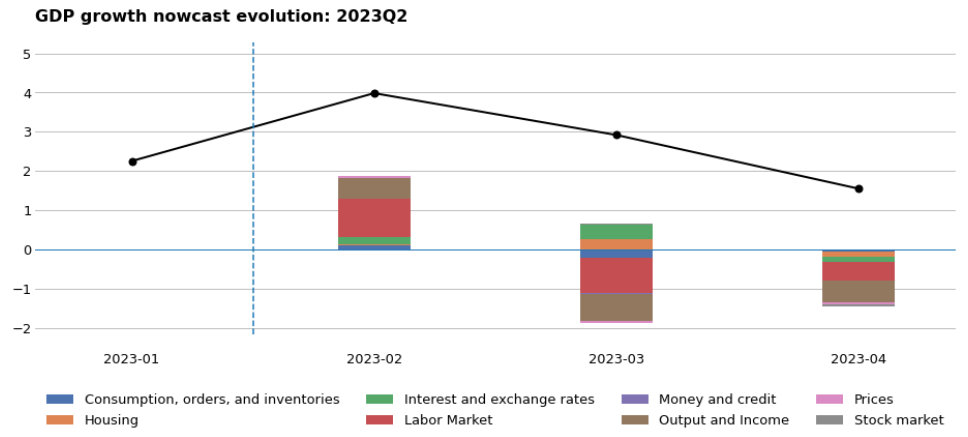
Data Srouce: FRED database
Lattent Factor for Economic Condition Indeces
Another valuable aspect of the nowcasting model, which I believe is particularly useful from an investment perspective, is the extraction of key latent factors from the vast array of economic variables. The economy is a complex system, with different factors impacting various sectors of the financial markets. No single or few economic indicators can perfectly meet our investment needs. The nowcasting model provides a flexible tool for us to extract insights in a tailored manner.
We have the opportunity to design a suitable structure for extracting investment insights in the form of latent factors. For instance, we can group economic indicators based on their influence on various perspectives such as economic growth, monetary policies, and more. Additionally, we can explore lead-lag effects among different indicators and incorporate these dynamics into the model. For example, we might discover that energy consumption generally precedes changes in industrial output. All of these dynamics can be incorporated into one or a couple of models, based on our preferences.
These latent factors can be transformed into economic condition indexes that represent the overall movements of specific aspects of the economy that we believe relavant in investment. A thoughtfully designed economic index that effectively summarizes a particular aspect can serve us well in our investment endeavors.
In the chat below, I have plotted two indexes from the previous toy example for illustrations. The global factor represents a general condition of the economic operation as it loads on all economic indicators. On the other hand, the Labor Market factor specifically loads on labor-related indicators such as the unemployment rate.
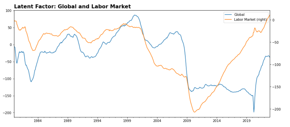
With these economic condition indexes at our disposal, it remains our choice to directly use them to forecast the performance of certain securities or exercise caution and categorize market regimes based on the index, leading to further research opportunities etc…
The possibilities are abundant while falls beyond the scope of our current discussion. For now, our discussion comes to a conclusion. Hopefully you find it interesting :)
Reference
- Banbura, Giannone & Reichlin(2010): Nowcasting
- Banbura & Modugno (2010): Maximum Likelihood Estimation of Factor Models on Datasets with Arbitrary Pattern of Missing Data
- Bok, Caratelli, Giannone, Sbordone & Tambalotti (2018): Macroeconomic Nowcasting and Forecasting with Big Data
- Chad Fulton’s Blog: Large dynamic factor models, forecasting, and nowcasting