From Volatility to Maximum Drawdown
- Introduction
- Maximum Drawdown: The Way to Approach
- Maximum Drawdown Greek: A Simulation View
- Reference
Introduction
In the realm of risk measures, volatility stands out as a star player, and with good reason. It has deep roots in asset pricing theories, intricately connected to the concepts of both risk and reward; It lends itself to reliable estimation and forecasting in real-world applications. It bears favorable analytical properties hence can be extensively analyzed and efficeintly controlled in portfolio construction …
The advantages of using volatility to gauge risk are plentiful. While it may not align perfectly with the traditional view of risk, it encompasses both unexpected losses and gains, recognizing the latter as a “nice surprise.”
Maximum Drawdown takes the center stage as one of the most popular risk measures focusing on downside of an investment. Investors pay keen attention to it as it represents the worst possible scenario one can encounter on an investment: buying at peak and exiting at trough. As such, it finds its place in all forms of investment reporting materials.
In this blog, let’s embark the journey to explore maximum drawdown. Our initial section touch upon ideas to approach this measure despite tis less-than-ideal analytical properties. Subsequently, we examine the crucial factors that influence Maximum Drawdown through simulations, starting from the standard IID Gaussian and extending into the intricate realm of time dependence and non-Gaussian distributions. Many insights in the second section are drawn from the informative article Van Hemert, Ganz, Harvey, Rattraym Martin & Yawitch (2020): Drawdowns
Maximum Drawdown: The Approach
The definition and ex-post calculation of Maximum Dradwon (\(MDD_t\)) are unambiguous. Given the time series of net value on a strategy or security (\(P_t\)), we begin by identifying the peak (\(M_t\)) up to each point t. From there, it’s straightforwad to calculate the drawdown (\(D_t\)) as the loss compared to that cumulative peak for each moment. The shapest drawdown observed is what we term as maximum drawdown.
\[\begin{aligned} M_t &= \max_{\mu \in [0, t]}{P_{\mu}} \\ DD_t &= \dfrac{P_t - M_t}{M_t} \\ MDD_t &= \min_{\mu \in [0, t]}{DD_{\mu}} \end{aligned}\]It’s clear that the characteristics of the return distribution, as well as the time dependence and the duration of return occurrences, are of great importance. An extended investment horizon and a consecutive string of losses are more likely to trigger severe drawdowns. The Maximum Drawdown is thus a random variable jointly determined by the stochastic return process and the investment horizon.
Ideally, we would derive the distribution of the Maximum Drawdown in terms of the return process and horizon, conduct study on the distribution thoroughly, and then use this knowledge for portfolio construction and risk management. Unfortunately, such a comprehensive approach is generally unfeasible for the Maximum Drawdown.
There is generally no closed-form solution to describe the distribution of Maximum Drawdown. Magdon-Ismail et al (2004) derived the cumulative distribution function of Maximum Drawdown under the assumption that the net value of investment follows a Brownian motion with zero drift. However, even this cumulative distribution function, under quite ideal assumptions, is too complex for intuitive discussions or inclusion in portfolio optimization. Moreover, calculating the ex-ante Maximum Drawdown of a portfolio requires more than the Maximum Drawdown of each constituent; it calls for forecasting the return series for every constituent within the universe (N*T), an impractical endeavor.
Nevertheless, the hope is not lost. Despite these challenges, we can circle around and address Maximum Drawdown indirectly. For instance, during portfolio optimization, we can penalize characteristics that tend to increase the magnitude of the Maximum Drawdown while being easier to incorporate, such as negative skewness or excessive kurtosis.
Additionally, while obtaining a closed-form function to describe the distribution of the Maximum Drawdown is elusive, designing investment policies to control it is comparatively more attainable. Grossman & Zhou (1993) offered an optimal investment policy under Gaussian assumptions, allowing investors to achieve optimal expected utility growth with a hard constraint on Maximum Drawdown through dynamic adjustments in the holdings of risky assets.
To delve deeper into the practical application of these efforts. We would appreciate to have some impressions about relavant factors and their impact on Maximum Drawdown. This is precisely what we aim to explore through simulations in the next section.
Maximum Drawdown Greek: A simualtion view
In the absence of an analytical description of the Maximum Drawdown distribution, we turn to the tool of simulation. Swinging the hammer of simulation, we can get a sense of how the probability of reaching a specific Maximum Drawdown level is influenced by some key relavant attributes.
Setting the Baseline
Following Van Hemert et al. (2020), we start with a baseline return generation process featuring a 0.5 Sharpe ratio and 10% volatility. This monthly return is simulated over a 10-year period for 100,000 times to build the empirical distribution of the maximum drawdown. The probabilities of breaching Maximum Drawdown thresholds of 1, 2, 3, and 4 multiples of volatility (corresponding to -10%, -20%, -30%, and -40% volatility) are found to be 97.%, 43%, 9.9%, and 1.5%, respectively.
Building upon this baseline, we introduce variations in volatility, Sharpe ratio, time horizon, and incorporation of time dependence, along with deviations in higher moments to assess their impact. We aim to get some sense on how these changes influence the probability of breaching Maximum Drawdown thresholds expressed as multiples of standard deviations (sigmas). As we delve into the details below, we discover that a lower Sharpe ratio, an extended investment horizon, higher auto-correlation in returns and volatility, and increased kurtosis all contribute to larger Maximum Drawdowns.
The ‘Good Old’ IID Gaussian
Let’s commence our journey in the familiar world of IID Gaussian, where mean and variance solely determine return generation. In this scenario, only three factors influence Maximum Drawdown: mean, variance, and investment horizon. In the three charts below, we investigate how changing volatility, Sharpe ratio (as a proxy for mean), or time horizon while keeping the other two constant impacts Maximum Drawdown.
An intriguing observation is that when we express Maximum Drawdown thresholds as multiples of volatility, variations in volatility have almost no impact on the probabilities of breaching these thresholds. The slight downward slope can be attributed to the compounding nature of return aggregation. This suggests that imposing constraints on volatility alone can effectively limit Maximum Drawdown in the IID Gaussian scenario. It also supports Van Hermer et al.’s (2020) choice to express Maximum Drawdown thresholds as multiples of volatility.
On the other hand, it’s unsurprising to see that probabilities of breaching Maximum Drawdown thresholds rise as Sharpe ratio decreases or investment horizon lengthens.

Higher Moments
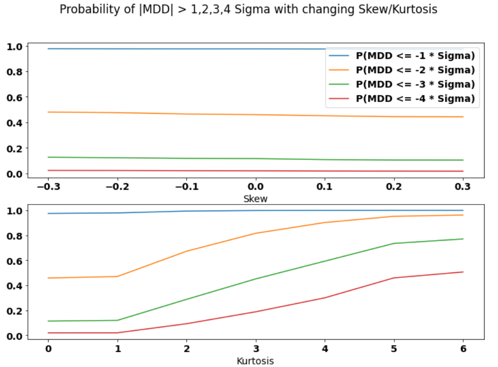
In reality, investments rarely follow the IID Gaussian. Deviations in distribution or time dependence are more commonly encountered. To mimic these differences in higher moments of the distribution, we employ the Gram-Charlier expansion to introduce skewness and kurtosis deviations to the baseline case. We then assess their impact on Maximum Drawdown.
To ensure a well-defined distribution, we vary skewness from -0.3 to 0.3 and excess kurtosis from 0 to 6, aligning the mean and variance with the baseline case for a fair comparison. Within this range, changes in skewness don’t significantly impact Maximum Drawdown, whereas increases in kurtosis lead to a substantial rise in Maximum Drawdown. However, this doesn’t imply that skewness doesn’t influence Maximum Drawdown. Our simulations are restricted to a relatively narrow range, making it challenging to explore the full range of skewness’s impact.
Time Dependence
Last but by no means least, we introduce the dimension of time dependence to both returns and local volatility within the baseline case.
In particular, we simulate returns with auto-correlation ranging from -0.5 to 0.5 using the following formula, where the parameter \(\rho\) signifies the auto-correlation added. As shown in the first chart below, increasing the auto-correlation corresponds to an increase in the probabilities of reaching corresponding Maximum Drawdown thresholds.
\[r_t = (1-\rho) \mu + \rho r_{t-1} + \sqrt{1 - \rho ^ 2} \sigma\]To emulate the volatility clustering seen in many asset classes, we use an ARCH(1) process. The larger the parameter \(alpha_1\), the more pronounced the volatility clustering becomes. Similarly, we observe an increase in probabilities with greater volatility clustering.
\[\begin{aligned} r_t &= \mu + \sigma_t e_t \\ \sigma_t^2 &= \alpha_0 + \alpha_1 r_{t-1}^2\\ e_t &\sim N(0, 1) \\ \sigma^2 &= \dfrac{\alpha_0}{1-\alpha_1} \end{aligned}\]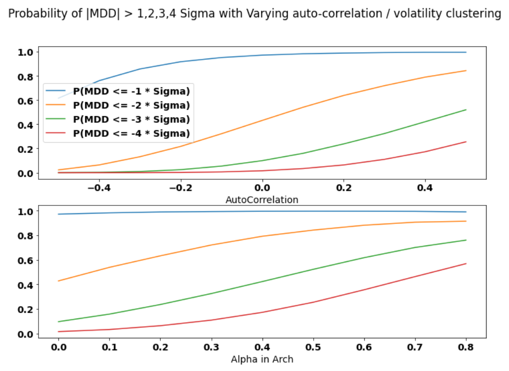
Reference
- Van Hemert, Ganz, Harvey, Rattraym Martin & Yawitch (2020): Drawdowns
- Magdon-Ismail, Atiya, Pratap & Abu-Mostafa (2004): On the Maximum Drawdown of a Brownian Motion
- Grossman & Zhou (1993): Optimal Investmetn Strategies For Controlling Drawdowns
- Palomar’s Slide on Portfolio Optimization with Alternative Risk Measures