The Adjustment for Luck!
- Those Factors shrink out of sample
- A multiple testing problem
- A Resample Procedure to account for luck
- And More
- Reference
Those Factors Shrink out of sample
As Nobel Laureate Ronald Coase once said: “If you torture data long enough, it will confess to anything”.
It starts with the million dollar question in finance and investment - What factors explain security expected return? Ever since the 90s when Fama and French’s empirical work on the 3 factor model unleashed a new era of empirical asset pricing, hundreds (if not thousands) of factors have emerged in academic and industry research, each claiming to predict cross-sectional or time-series security returns. While despite this plethora of factors (John Cochrane calls it a factor zoo), predicting security expected returns in real-world investments remains a challenging task. Many of these factors, despite demonstrating strong in-sample performance (which lead to their publication), significantly underperform out-of-sample.
For example, Pontiff and McLean (2016) examined the out-of-sample and post-publication performance of around 100 cross-sectional factors from academic research. Unfortunately, they found that, on average, factor returns shrank by 26% out-of-sample and 58% post-publication. Hou, Xue & Zhang (2020) further exapeded this exercises to a total of 452 factors published and found that for as much as 65% of them, t-statistics drop below 2 out of sample.
Let’s leave alone all the dicussion and debates about potential replicating crisis in asset pricing literature for the moment, deteriorating out sample performance was indeed observed for a lot of factors published. Why is it the situation? The reasons behind this performance deterioration out of sample are numerous and complex, each deserving thorough research and discussion. In this blog we will try to discuss about one particularly interesting aspect of the problem: those “lucky factors” selected only because of test multiplicity from a large number of candidate factors. They would not continue the luck in a new sample!
Obviously, to improve our chance of expected return prediction, we hope to select factors that genuinly means something and are likely to maintain their predictive power out of sample. These lucky factors are what we hope to avoid in the modeling of expected return. To this goal, how can we adjust our factor research framework for the existence of lucky factors and how good should one factor perform so that we are comfortable to declare its statistical significance accounting for the turbulance of luck. That’s the question that we hope to discuss in this blog. Specifically I hope to introduce to your attention the resample statistical procedure from paper “Lucky Factor” (Harvey & Liu, 2021). Given a pool of candidate factors, such a statistical procedure is quite helpful in evaluating marginal improvement on adding factors to existing factor models while also accounting for the lucky factor problem.
A Multiple Testing Problem
So, what is this ‘lucky factor’ problem and where does it come from? In short, it originates from the exhaustive efforts of data mining (or data snooping) conducted on financial data set without accounting for the test multiplicity arised. Whenever a factor is identified by an extensive or exhaustive search, there is the danger that its good performance is not from real prediction ability but rather just luck.
In factor research, we infer an argument about the population (i.e., what is the expected return of the factor?) based on sample observations (i.e., the performance of the factor in this sample). Probability is our bridge for nagivating between the two. Statistical lemmas like Law of Large Number and Hoeffding Inequality assure us that as long as the observations are sampled independently from the population, the sample performance should not deviate significantly from the true performance of the factor given a sufficient number of observations N.
\[\begin{aligned} \hat{Performance(F)} &\rightarrow N(Performance(F), \dfrac{1}{N}\sigma^2)\\ P(|\hat{Performance(F)} &- Performance(F)| > \epsilon) <= 2e^{-2\epsilon^2N} \\ \end{aligned}\]While, as long as we do not have the full population, there is still a probability inversely proportional to N of a larger-than-expected gap between the true expected return and the sample estimation. Thus, we accept an inevitable possibility of false discovery when recognizing the significance of a factor.
Typically in factor research, we test the null hypothesis that the expected return of the factor is zero. If the null hypothesis contradicts the sample performance, indicating a rare event under the null hypothesis, we reject the null hypothesis and consider the factor to have a significant expected return. In this process, p-value is calculated and compared against a threshold to determine how compatible the null hypothesis is with the data. In the context of single hypothesis testing, a 5% p-value threshold means there is at most a 5% risk of false discovery if we deem the factor significant.
However, this logic falters when many factors are tested in a horse-racing style research. Imagine identifying one factor with a p-value of 5% — right at our threshold — after 399 unsuccessful attempts. The risk of accepting this 400th factor is no longer 5%. That is because, even if all 400 factors share expected return of zero, randomness alone would give a probability greater than 99% of finding at least one factor with a p-value below 5% in the sample — the ‘lucky’ factors. Identifying one factor out of 400 trials is insufficient to contradict the null hypothesis since “none of the 400 factors tried has significant in-sample performance” is not an accurate description of the null hypothesis due to the randomness embeded.
Unfortunately, this is more or less what we face in factor research. In the sparkling financial markets, hundreds of thousands of researchers have tested countless factors for predictive power using similar data sets. They generally use a p-value threshold of 1% or 2.5% or 5% under the single hypothesis test framework, leading to significant multiple testing issues. With so many factors tested, a factor showing strong in-sample predictability by the standards of single-factor testing is often the result of random chance rather than genuine predictive power.
Hence it’s really not surprising to see the deterioration of out sample performance. We have these lucky factors in the respository of published factors!
A Resample Procedure to account for luck
Now with some better understanding about the ‘lucky factor’ problem and its origins, how can we address it? Thre are multiple angles to approach such a question.
Harvey and Liu (2021) provide one viable solution from the perspective of frequentist approach. They suggest to use max statistics to adjust for test multiplicity and design a statistical procedure combining orthogonalization and resampling to enforce the null hypothesis in the context of test multiplicity in regression analysis. This procedure works with various types of regressions, whether time series, panel regression, or Fama-Macbeth regressions. Even better, it can be applied to an existing model to select additional factors, enhancing it by measuring marginal improvement after accounting for luck.
Suppose we have variable Y, the observed return to predict, and X, the candidate factors to use. Based on previous research, we have already selected k significant factors from X to use. The following four steps help us continue the selection from the remaining factors (K+1 to M) while considering test multiplicity. The core idea of this procedure is to build the empirical distribution of the null hypothesis — what would the performance look like if all our candidate factors had zero expected return — and compare it to the true performance in the sample for decision.
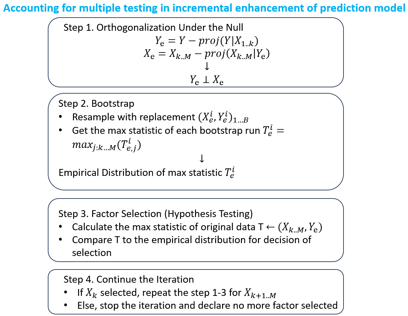
Firstly, obtain the reidual \(Y_e\) of \(Y\) after projection onto selected factors \(X_{1...K}\). \(Y_e\) represents the proportion of return that the current model fail to predict and what we aim to improve upon. If starting from scratch, use \(Y\) as \(Y_e\), in which case, all of the return is the target to improve. After orghonalizing the remaining candidate factors with respect to the \(Y_e\), the null hypothesis is established: \(X_e\) is orthogonal to \(Y_e\), indicating no predictive power of \(X_e\) on \(Y_e\) in the orthogonalized sample.
The second step is about learning the empirical distribution of lucky factors by sampling from the orthogonalized dataset. For each sampling iteration i of \((X_e^i, Y_e^i)\) we draw. A chosen statistic such as t-statistic, p-value or R square is calculated for all candidate factors and the best statistic of all (\(T_e^i\)) is stored. Since we have already carved out all the prediction power in the dataset, a good \(T_e^i\) would be a lucky factor in this resampled set. We can get the empirical distribution of this max statistic by sampleing for multiple iterations.
This distribution of lucky factors serves as the null hypothesis distribution where all factors have zero expected return. With a proper description of the null hypothesis, we can calculate the max statistic from the original data and compare it against the distribution of lucky factors to decide on selection. As deliberately designed in the orthogonalization step, the difference reflects predictive power accounting for luck. If the max statistic stands out even compared to the distribution of lucky factors, we would have more confidence in its true predictive power beyond luck.
Such steps can be repeted to continue the selection of factors until the point where we are no longer satisfied on the comparison between the real max statistic and the empirical distribution of lucky factors. And it concludes all the factors we are comfortable to add under the procedure with attention paid to lucky factors.
And More
It’s reassuring to know that we have tools to address, or at least mitigate, the lucky factor problem. To me, this resample precedure is particularly helpful for at least two reasons. Firstly, it offers a practical method to account for multiple testing in the context of incrementally enhancing a prediction model. Secondly, having the empirical distribution of the max statistic at our disposal allows us to gauge the magnitude of lucky factor performance that can emerge in a given sample. In fact, storing more than just the max statistic from each resampled dataset can provide valuable insights for risk management.
However, like all models, this procedure has its limitations. It’s definitely a good idea to discuss them before concluding.
Firstly, the true number of factors experimented is generally unknown and likely much larger than we assume. For instance, when selecting factors from a pool of candidate factors, it is probable that these candidates are themselves results of extensive, horse-racing style research. Even if we begin our exercise from scratch, merely reading articles about factors might expose us to the test multiplicity made by the authors unconsciously. Some would suggest modeling the t-statistic of documented factors as a truncated distribution to infer the number of experiments involved. While viable, this approach does introduce more reliance on assumptions.
Additionally, this procedure treats all candidate factors equally, evaluating them solely based on their sample performance. Ideally, we would give more credits to factors with solid theoretical foundations, as these factors embody the wisdom derived from structural modeling or correlated datasets, which can improve our predictive accuracy. The sampling method doesn’t actually support this kind of differentiation well. While we can take theory-backed factors as selected and build from there, imposing any intricate structure might be better suited to a Bayesian framework, which allows for modeling them in the prior. As for the Bayesian approach to modeling expected return, we’ll leave that for discussion in the next blog.
Reference
- Harvey & Liu (2021): Lucky factor
- Pontiff & McLean (2016): Does Academic Research Destroy Stock Return Predictability?
- Hou, Xue & Zhang (2020): Replicating Anomalies
- White (2000): A Reality Check for Data Snooping