The “Maximum Diversification Frontier”
- Introduction
- MD Portfolio: the theoretical underpings
- How’s the performance for the past decade
-
Introduction
In the previous blog post The Conviction Pyramid of Portfolio Construction, we embarked on an exploration on various portfolio construction methods, each tailored to different levels of market information availability. One such method we discussed (and I found very handy in quite some applications) is the Maximum Diversification (MD), which aims to maximize diversification in terms of correlation. It is a direct application of the notion diversification for efficient risk premium harvest and provides much more flexibility in integrating optimization constraints compared to its closely related couterpart Risk Parity (RP).
Expanding our exploration of MD, this blog post will take a closer look at its application in strategic asset allocation. We will examine the underlying assumption of consistent long-term balance between risk and return that underpins MD. More importantly, we will explore MD at various volatility targets to construct an achievable “Maximum Diversification Frontier” and examine its performance at major markets like US, Eurozone, Japan, and China.
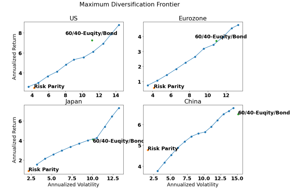
The resulting “Maximum Diversification Frontier” showcases an upward frontier, depicting the increasing realized risk and return at corresponding risk targets. Hence as a parrallel of the efficient frontier (probably also intersect at some points), I have the blog named as “Maximum Diversification Frontier”.
MD Portfolio: the theoretical underpings
Let’s go for diversification !
Diversification has long been regarded as a fundamental principle since the advent of modern portfolio theory. The renowned Nobel Prize laureate Harry Markowitz is reported to have said “diversification is the only free lunch” in investing. The prevailing belief is that in a rational market over long term, only non-diversifiable systematic risks (those covary with stochastic discount factor, consumption…etc) are rewarded with expected returns. Therefore, efficient diversification, which reduces idiosyncratic risk, is considered crucial for enhancing risk-adjusted returns (at least in an unconditional context without additional information).
In line with this concept, Maximum Diversification (MD) is introduced to exploit the imperfect correlations among securities within the investment universe. More formally, MD seeks to maximize the diversification ratio, which is defined as the weighted average volatility over the portfolio volatility. In cases where all securities move in perfect harmony, this ratio can reach a maximum value of 1.
\[\begin{aligned} Max_{w} & \dfrac{w^T \sigma}{\sqrt{w^T \Sigma w}} \\ w^T 1 &= 1 \end{aligned}\]By targeting the diversification ratio as the optimization objective, MD overweights securities that exhibit low correlations with others, resulting in a straightforward and intuitive implementation of the diversification principle.
The optimal assmuption of risk return consistency?
Is there any further rationale behind MD beyond its direct implementation of diversification? Absolutely! Particularly in the context of strategic asset allocation. In our previous discusion, we observed that for a portfolio to be MD, the following conditions must hold for every pair of securities within the portfolio:
\[\begin{aligned} \dfrac{1}{\sigma_i} \dfrac{\partial \sigma_p}{\partial w_i} &= \dfrac{1}{\sigma_j} \dfrac{\partial \sigma_p}{\partial w_j} \end{aligned}\]As a contrast, the maximum sharpe ratio portfolio requires the following conditions
\[\begin{aligned} \dfrac{1}{r^{e}_i} \dfrac{\partial \sigma_p}{\partial w_i} &= \dfrac{1}{r^{e}_j} \dfrac{\partial \sigma_p}{\partial w_j} \\ \end{aligned}\]Combining the two, we can see that MD is essentially equivalent to the Maximum Sharpe Ratio portfolio if the expected return is linearly proportional to volatility for every security in the investment universe. With MD, we’ve touched the holy grail (at least in some degree)!
This balance relationship between return and volatility is not some crazy illution within asset classes. While there is not a definitive conclusion if asset classes should share the same sharpe ratio. The assumption that asset classes have comparable return volatility ratio is generally recogonized as sound, making MD a reasonable choice in asset allocation.
Asset classes (equity, fixed income, commodity, etc …) are generally represented as well diversified portfolios. Over the long term, investors tend to flock to asset classes with extraordinary returns compared to their volatility, as they seek risk-adjusted returns. This influx of capital drives up the price of the asset class, thereby reducing its risk-adjusted return to a comparable level with other asset classes.
It is generally the case for the past 20 years (bear with the poor drawing of the green line)
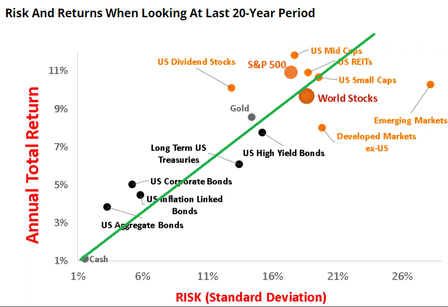
Source: Bankeronwheels.com
It also aligns with the long term capital market expectation forecast from institutional investors, such as the one below from BlackRock.
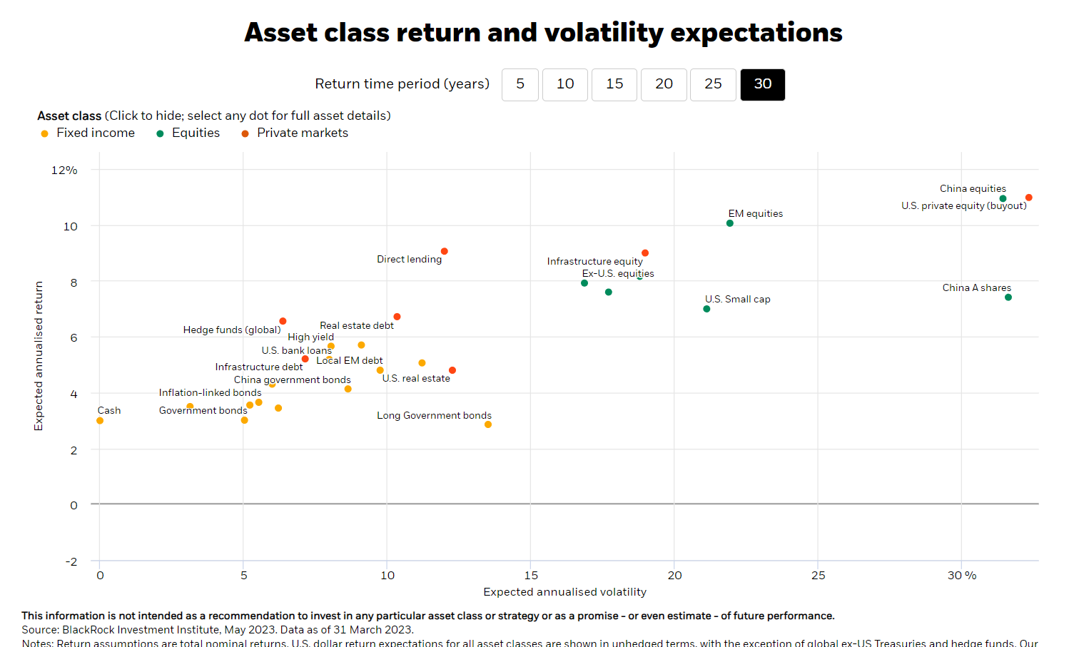
Source: www.blackrock.com
In both cases, asset classes cluster around a straight line, indicating that they share a comparable return-to-volatility ratio.
The frontier part
So MD is a good choice in asset allocation. What about the “frontier” aspect mentioned in the blog title?
It stems from the remarkable flexibility of MD optimization. Within any feasible set of the universe, there will always be at least one portfolio that maximizes the diversification ratio, given that it is a relative metric. This inherent feature allows us to easily incorporate various optimization constraints into MD optimization.
Among these constraints, the volatility target aligns particularly well with MD optimization. This portfolio construction approach is rooted in the idea of first positioning ourselves within the realm of acceptable risk and then effectively utilizing that risk through diversification.
By applying MD optimization with volatility targets, we can generate a set of well-diversified portfolios for any given volatility target, thereby forming a “Maximum Diversification Frontier,” as demonstrated in the chart at the beginning of the blog post. From my perspective, this frontier offers tremendous convenience in providing a comprehensive range of options that can align with the utility function of client or specific product madates
How’s the performance for the past decade
Let’s examine the performance of such an idea in the markets of US, Eurozone, Japan and China.
In the following bactkest analysis, market value weighted equity indexes, aggreagate bond indexes and commodity indexes from S&P are used to represent each asset class. All index levels are stated in the local currencies in corresponding markets to avoid FX turbulence.
It is worth mentioning that these indexes are selected because their return data is freely available on S&P’s website. However, it is unfortunate that their data covers only the past decade, which, from the perspective of strategic asset allocation, can be considered a relatively short period. Nevertheless, we can still provide a concise overview of the idea.
In each market, I have optimized multiple MD portfolios with volatility targets ranging from 3% to 13% with the following set up. While other constraints related to risk and regulation can also be incorporated, for the purpose of illustration, we will keep the discussion focused.
\[\begin{aligned} Max_{w} & \dfrac{w^T \sigma}{\sqrt{w^T \Sigma w}} \\ w & > 0 \\ w^T 1 &<= 1 \\ \sqrt{w^T \Sigma w} & = \sigma_{target} \end{aligned}\]The covariance matrix in each market is estimated using an exponential weighted sample covariance matrix based on daily returns with a halflife of 126. The portfolios are optimized and rebalanced quarterly, starting from 2015 (with the first two years allocated for parameter estimation) until 2023.
The final results of all backtests are displayed in the chart at the beginning of the blog post, along with detailed performance presented in the table below. The “MD @ x Risk” represents the MD portfolio optimized at a volatility target of x with Risk Parity and 60/40 portfolio for the same period as contrast. As anticipated, MD proves to be a reasonable solution for strategic asset allocation. I would like to emphasize two key points:
-
The volatility target effectively constrains the volatility of all portfolios close to their respective volatility targets (If we look for 6% of volatility, we get 6% realized volatility). By utilizing only local information during each rebalancing, we are able to manage long-term volatility effectively. This outcome can likely be attributed to the clustering and long-term mean reversion characteristics that are prevalent in volatility.
-
As we increase other volatilityu target, the final expected return also exhibits a relatively stable growth pattern along with the realized volatility. In my view, this indirectly indicates that risk is being utilized efficiently. Each additional level of risk taken has the potential to yield further rewards.
In my perspective, the MD approach with risk targets serves as an exceptional foundation for asset allocation, especially suited for Asset Only investors who don’t have stringent constraints regarding matching durations or cash flows. This approach allows us to position ourselves at the desired risk level and efficiently utilize risk through diversification.
| US | Eurozone | Japan | China | |||||
|---|---|---|---|---|---|---|---|---|
| Annualized STD | Annualized Ret | Annualized STD | Annualized Ret | Annualized STD | Annualized Ret | Annualized STD | Annualized Ret | |
| MD @ 3% Risk | 3.59 | 2.61 | 3.47 | 0.74 | 3.19 | 1.55 | 3.08 | 3.77 |
| MD @ 4% Risk | 4.77 | 3.01 | 4.52 | 1.06 | 4.20 | 2.13 | 4.10 | 4.17 |
| MD @ 5% Risk | 5.89 | 3.66 | 5.55 | 1.43 | 5.22 | 2.57 | 5.11 | 4.54 |
| MD @ 6% Risk | 7.01 | 4.13 | 6.57 | 1.83 | 6.25 | 2.97 | 6.12 | 4.89 |
| MD @ 7% Risk | 8.06 | 4.81 | 7.59 | 2.25 | 7.29 | 3.34 | 7.13 | 5.18 |
| MD @ 8% Risk | 9.01 | 5.32 | 8.61 | 2.64 | 8.34 | 3.68 | 8.14 | 5.43 |
| MD @ 9% Risk | 10.17 | 5.55 | 9.57 | 3.19 | 9.40 | 4.00 | 9.16 | 5.56 |
| MD @ 10% Risk | 11.29 | 6.10 | 10.63 | 3.45 | 10.52 | 4.27 | 10.16 | 5.64 |
| MD @ 11% Risk | 12.49 | 6.91 | 11.67 | 3.97 | 11.49 | 5.42 | 11.11 | 5.90 |
| MD @ 12% Risk | 13.44 | 7.86 | 12.60 | 4.55 | 12.37 | 6.46 | 12.03 | 6.21 |
| MD @ 13% Risk | 14.35 | 8.77 | 13.29 | 4.76 | 13.20 | 7.33 | 12.92 | 6.50 |
| RP | 4.27 | 2.50 | 4.15 | 0.57 | 2.16 | 0.89 | 1.60 | 4.78 |
| 60/40-Equity/Bond | 11.16 | 7.24 | 10.92 | 3.71 | 10.02 | 4.12 | 15.10 | 6.50 |
Reference
- Choueifaty & Coignard (2008): Toward Maximum Diversification