The Practical Side of Black-Litterman and More
- Introduction
- The Practical Side of Black-Litterman
- More on Expected Return Forecast with Black-Litterman
- Reference
Introduction
Forecasting expected return is a rewarding yet challenging endeavor. One shot to tilt the odds in our favor a bit in this battle is probably to take into account as much relavant information as possible. In such cases, a reliable method to weave together these information of distinct categories and forms becomes quite crutial.
The Black-Litterman model stands as a dependable solution in this quest. As we explored in the previous blog (Anchor Your Forecast the Bayesian Way), the model serves a dual role. On one hand, it safeguards our baseline by anchoring the refined estimates to a benchmark portfolio. On the other, it opens the door to upward potentialy by allowing us to seamlessly integrate a multitude of forecats from various models, all within a risk-aware framework.
This model serves as an excellent starting point in our expedition to refine expected return forecasts. While there’s still a vast landscape to explore ahead! Within this blog, let’s embark on a deeper dive into the practical side of the Black-Litterman model and close with a causual chat on the two perspectives of the framework just mentioned.
The Practical Side of Black-Litterman
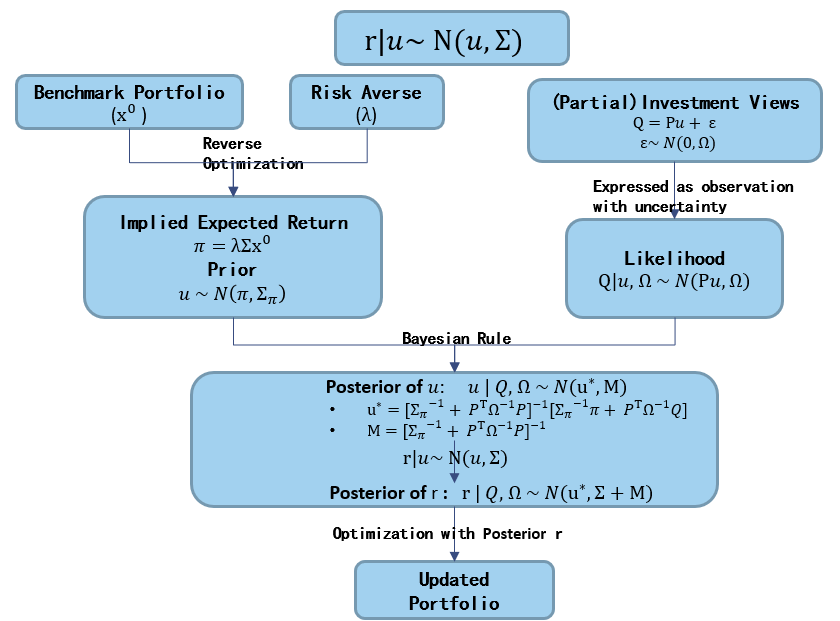
Let’s pick up where we left off in our exploration of the Black-Litterman model in the previous blog (Anchor Your Forecast the Bayesian Way). Without too many assumptions placed so far, we get a refined forecast that combines all original forecasts and prior in the form of posterior.
\[\begin{aligned} \mu^{\star} &= (\Sigma_{\pi} + P^T\Omega^{-1}P)^{-1}(\Sigma_{\pi}^{-1} \pi + P^T\Omega^{-1}Q) \\ M &= (\Sigma_{\pi} + P^T\Omega^{-1}P)^{-1} \end{aligned}\]This is a general framework, with which, we are free to feed in all kinds of forecasts (prior and likelihood) within the Gaussian world. However, applying such a general model demands significant estimation in application. Consider, for instance, the two matrices that quantify uncertainty (\(\Sigma_{\pi}\) and \(\Omega\)) alone, we have \(N^2 + K^2\) parameters to estimate. (N and K refers to number of securities in the universe and number of original forecast respectively).
To streamline the estimation process and mitigate model risk originated from large number of estimations, a lot of techniques with further restriction upon the Gassuan assumption are applied in application. Let’s look into some of these techniques that faciliate the practical application of the framework.
The Black Litterman Tau
One authentic assumption made by Black & Litterman themselves is that the covariance matrix measuring uncertainty around prior (\(\Sigma_{\pi}\)) is proportional to return covariance matrix (\(\Sigma_{\pi} = \tau \Sigma\)). Remeber that, to maintain a solid baseline, the prior mean is extracted from reverse optimization of benchmark portfolio wihout clearly defined uncertainty. This one additional assumption instantly free us from the estimation of \(N^2\) somewhat vague parameters.
Certainly, it is not the ‘correct and accurate’ assumption, while it does capture some key points from the full picture and significantly eases the tension on estimation. In practice, higher volatility in security returns generally translates to greater uncertainty in estimating expected returns.
With the tau factor in play, we arrive at the standard Black-Litterman estimatior in the following form:
\[\begin{aligned} \mu^{\star} &= (\tau \Sigma + P^T\Omega^{-1}P)^{-1}((\tau \Sigma)^{-1} \pi + P^T\Omega^{-1}Q) \\ M &= (\tau \Sigma + P^T\Omega^{-1}P)^{-1} \end{aligned}\]Now, the scaling factor \(\tau\) is all required to determine the unceratainty around prior. Typically, \(\tau\) is assigned heuristically with a small value close to 0 as “uncertainty in the mean is much smaller than the uncertainty in the return itself” (Black & Litterman (1992)).
Broadly speaking, this argument aligns with other methods proposed to set \(\tau\). Whether to take the uncertainty as sampling error (\(\tau = \dfrac{1}{T}\)) or to infer it from holding in risky asset in reference portfolio (\(\tau = \dfrac{1}{w_{risky}} - 1\)). These approachs generally lead to a \(\tau\) at the range within 0 and 0.1. Walters (2013) provides a very comprehensive review about the parameter \(\tau\).
The Subjective Omega
With \(\tau\) neatly defining uncertainty around the prior, let’s take a more detailed look into the uncertainty around likelihood. The goal is to embrace a wide array kinds of investment views in the form of likelihood.
It is relatively straightforward to set the uncertainty around investment views generated from statistical models. Forecasting errors, such as the residual variance in a regression, naturally find their place in this context. However, similar to prior mean extracted from reverse optimization, it is indirect to deal with investment views that don’t emerge from quantitative methods and lack forecast errors (i.e., forecasts from subjective judgment). Incorporating such investment views demands extra efforts and considerations.
Drawing inspiration from Black and Litterman’s approach to model prior uncertainty, we can extend a similar principle to other investment views — linking their uncertainty to return variance. After all, it’s the relative level of uncertainty that truly matters. For a subjective investment view k expressed as a linear portfolio (\(p_k\)), we can assume that the uncertainty is scaled based on the portfolio variance.
Now the question turn to the setting of \(\alpha\).
\[\begin{aligned} \omega_k &= \alpha P_k \Sigma P_k^T \end{aligned}\]It’s worth noting that when we apply this structure of \(\tau\) and \(\alpha\) to define the uncertainty around the prior and likelihood, the ratio of \(\dfrac{\tau}{\alpha}\) alone is sufficient to define our posterior mean (\(\mu^{\star}\)). It is the existence of posterior variance (M) that necessitates the seprate estimation of \(\tau\) and \(\alpha\).
\[\begin{aligned} \mu^{\star} &= (\tau \Sigma + P^T\Omega^{-1}P)^{-1}((\tau \Sigma)^{-1} \pi + P^T\Omega^{-1}Q) \\ &= \pi + \tau \Sigma P^T(\alpha P\Sigma P^T + \tau P\Sigma P^T)^{-1} (Q-P\pi) \\ &= \pi + \Sigma P^T (\dfrac{\alpha}{\tau} P\Sigma P^T + P\Sigma P^T)^{-1} (Q-P\pi)\\ M &= (\tau \Sigma + P^T\Omega^{-1}P)^{-1} \\ & = (1 + \tau)\Sigma - \tau^2\Sigma P^T (\tau P \Sigma P^T + \Omega)^{-1}P \Sigma \end{aligned}\]In practice, our primary focus often lies with the posterior mean rather than the posterior variance. This is probably the reason why such a simplification of \(\dfrac{\tau}{\alpha}\) is untilized in a lot of applications. It should be noted that, though retains many of the metris of the full scale framework, such a approach is no longer a full-fledged Bayesian framework.
There are also paths to uphold the sanctity of a full-fledged Bayesian framework with both posterior mean and variance defined.
Idozek Implied Confidence Level
Following the definition of \(\omega\) in \(\alpha\), Idozek(2007) introduced a remarkably intuitive method to infer \(\alpha\) from the percentage of confidence, as defined by the desired level of active deviation. This approach paints a clear picture of the translation from a subjective confidence level to \(\omega\).
Depending on our confidence in a particular investment view k, our refined posterior mean range from \(\mu^{\star}_{0}\) (in case of 0 confidence in the view/ \(\alpha \to \infty\)) to \(\mu^{\star}_{100}\) (in case of absolute confidence in the view \(\alpha \to 0\)). Correspondingly, our final portfolio built on the refined estimation would range from the most conservative portfolio \(x^{\star}_0\) to the most confident portfolio \(x^{\star}_{100}\).
\[\begin{aligned} \mu^{\star} &= \pi + \Sigma_{\pi}P_k^T(\Omega + P_k\Sigma_{\pi}P_k^T)^{-1} (Q-P_k\pi) \\ \mu^{\star}_{100} &= \pi + \tau\Sigma P_k^T (P_k\tau \Sigma P_k^T)^{-1}(Q - P_k\pi)\\ \mu^{\star}_0 &= \pi \\ x^{\star}_{100} &= (\lambda \Sigma)^{-1} \mu^{\star}_{100}\\ x^{\star}_0 &= (\lambda \Sigma)^{-1} \pi = x_0\\ \end{aligned}\]A confidence level (0% ~ 100%) can be defined in terms of the desired position (\(\hat{x}\)) between the two portfolios of \(x^{\star}_0\) and \(x^{\star}_{100}\).
\[\begin{aligned} confidence &= \dfrac{\hat{x} - x^{\star}_0}{x^{\star}_{100} - x^{\star}_0} \\ \hat{x} &= x^{\star}_0 + confidence * (x^{\star}_{100} - x^{\star}_0) \\ \end{aligned}\]This approach offers an intuitive and consistent means of expressing confidence. On one hand, it provides the flexibility to express confidence in percentage from 0% to 100%. On the other hand, this percentage of confidence is linearly proportional to our active weight and risk. As we move our confidence from 0% to 100%, the active weight progresses linearly from \(x^{\star}_0\) to \(x^{\star}_{100}\) and so does the active risk.
With the method in place, we simplify the estimation of \(\omega\) by linking it with a well defined percentange of confidence level. All we need is to back out the \(\omega\) that leads to this portfolio with desired deviation (\(\hat{x}\)). Walters (2007) provides an analytical solution of this portfolio leading even more simplied results.
\[\begin{aligned} \dfrac{1}{1 + \alpha} &= \dfrac{\hat{x} - x^{\star}_0}{x^{\star}_{100} - x^{\star}_0} = confidence \\ &\downarrow \\ \alpha &= \dfrac{1 - confidence}{confidence} \\ \omega_k & = \alpha p_k \Sigma p_k^T \\ \end{aligned}\]This approach can be applied systematically to all investment views lacking clearly defined uncertainty, effectively expanding the utility of the Black-Litterman framework to accommodate a wide array of investment perspectives, as long as subjective judgment on confidence level is available.
Haesen, Hallerbach, Markwat & Molenaar tau/alpha ratio
There are also ways to undertake the \(\dfrac{\tau}{\alpha}\) within a full fledged Bayesian framework. For application in asset allocation, Haesen, Hallerbach, Markwat & Molenaar (2017) introduced another modification that simplifies the Black-Litterman framework. They suggest assuming the availability of only absolute views on all securities and directly defining the ratio of \(\dfrac{\tau}{\alpha}\)instead of treating them as separate parameters. This strategic restriction transforms the matrix P into an identity matrix, resulting in significant simplification.
\[\begin{aligned} P &= I_N \\ &\downarrow \\ \mu^{\star} &= (1 + \dfrac{\tau}{\alpha})^{-1} (\pi + \dfrac{\tau}{\alpha}Q) \\ M &= (\tau^{-1} + \alpha^{-1}) \Sigma \end{aligned}\]Now within the mix of investment views, what truly matters is the ratio \(\dfrac{\tau}{\alpha}\). The weights assigned to these views in the refined forecast are linearly proportional to the ratio.
\[\begin{aligned} \alpha \to 0 (\dfrac{\tau}{\alpha} \to \infty)\\ \mu^{\star} &= Q\\ M &\to 0\\ \alpha = \tau (\dfrac{\tau}{\alpha} = \dfrac{1}{2})\\ \mu^{\star} &= \dfrac{1}{2} (Q + \pi) \\ M &= \dfrac{1}{2} \tau \Sigma \\ \alpha \to \infty (\dfrac{\tau}{\alpha} \to 0)\\ \mu^{\star} &= \pi \\ M &= \tau \Sigma \\ \end{aligned}\]More on Expected Return Forecast with Black-Litterman
The techniques we’ve explored thus far should sufficiently equip us to implement the Black-Litterman model. But before we wrap things up, I’d like to take one last pause to engage in a casual conversation about the journey we’ve been on.
The framework we’ve been dissecting so far is essentially a Gaussian Bayesian model, characterized by known variances and unknown means. Through this well-defined statistical expression, we can harmoniously combine forecasts on expected returns from diverse sources in a risk-aware manner. Among the multitude of forecasts in play, one is deliberately chosen to serve as the cornerstone, fitting the role of prior in the model, while all others find their place in the role of likelihood.
To draw an analogy with the construction of a building, refining expected returns is akin to erecting a structure. The setup of the prior is akin to laying the solid foundation of the building’s basement. Once this robust base is in place, we can efficiently construct additional levels on top of it by incorporating other forecasts in a risk-aware manner, much like building the different floors of the building.
The Baseline From Benchmark
In this journey, the prior, whether derived from a reverse optimization process or any other source, serves as the bedrock upon which we build our refined forecasts. It plays a dual role: first, as the “numeraire” against which all other forecasts are measured for reliability, and second, as a complete forecast in cases where other forecasts fall short.
Black & Litterman opted for an expected return extracted in reverse from the market portfolio as their foundation. This choice not only aligns with the market portfolio as starting point but also finds strong support theoretically in the CAPM model.
At the cost of losing a theoretical foundation like CAPM model, we do have the flexibility to choose any benchmark for prior extraction via reverse optimization. This approach makes perfect sense, given that portfolio performance and more are often evaluated relative to the benchmark portfolio. For instance, Haesen, Hallerbach, Markwat & Molenaar (2017) suggested using a risk parity portfolio as the basis for prior estimation in asset allocation applications.
It’s important to note that reverse optimization is not the sole method for defining the prior. We can choose other forecasts to serve in this role as well. In fact, within the framework, there isn’t a fundamental difference between the prior and the likelihood; they are both forecasts of expected returns with uncertainties around.
In my opinion, the ideal characteristics that distinguish one forecast as prior are twofold. First, the prior should span all the securities of interest within the universe, ensuring we have reliable estimates for every security, even when other forecasts are incomplete. Second, it should be a robust estimate, resistant to noise and drastic fluctuations, as these desirable qualities will carry over into the refined estimates.
Under these conditions, forecasts from various sources, such as those generated by multi-factor models, should make a good fit in the role of the prior as well.
The Refinement of Multiple Forecasts
With a solid foundation laid by the prior to safeguard our baseline, the prospect of incorporating additional forecasts to enhance performance becomes all the more exciting. Such a trial would likely improve the performance from various angles.
On one hand from the angle of financial market, countless factors exert their influence on expected returns across various timeframes and securities. However, owing to the inherent challenges of modeling and data limitations, there isn’t a single, unified model or framework capable of comprehensively addressing all these factors simultaneously. Instead, the approach to expected return forecasting often aligns with the wisdom of “divide and conquer.”
Consider the long-term horizon spanning decades, where fundamental variables like population growth and technological advancements play pivotal roles in forecasting asset class returns. As we zoom in to a horizon of a few years, factors tied to the business cycle, such as consumption and production, take the forefront in forecasting returns on asset classes, sectors, and more. As we further narrow our focus to shorter horizons, company-specific attributes become the linchpin for equity forecasting.
Likewise, the influence of various factors varies significantly across different types of securities. In the realm of equities, company-specific qualities like value and quality significantly impact pricing. Conversely, in the domain of debt, a distinct narrative unfolds, dominated by factors such as solvency and leverage. Meanwhile, within the domain of commodities, the ebb and flow of inflation rates wield substantial influence.
With specialized models tailored for specific horizons and selected subsets of securities, the rationale for combining forecasts becomes abundantly clear. By amalgamating insights generated from these diverse models, we assemble a more comprehensive view.
On the other hand from the angle of data science, the idea of combining forecasts aligns with a top-performing strategy in various data science competitions known as ensemble learning. Ensemble learning aims to merge multiple individual models into a more resilient meta-model, precisely what we aim to achieve here.
In our quest to combine forecasts from various models, we apply diverse models to overlapping yet distinct datasets, resembling a fusion of two popular ensemble learning strategies: stacking and bagging. By harnessing forecasts from varied datasets and models, there is indeed a rationale to expect a reduction in variance within the estimation, resulting in improved overall performance.
Reference
- Walters (2013): The Factor Tau in the Black-Litterman Model
- Walters (2007): The Black-Litterman Model in Details
- Idzorek (2007): A step-by-step guide to the Black-Litterman model
- Haesen, Hallerbach, Markwat & Molenaar (2017): Enhancing Risk Parity By Including Views