Anchor Your Forecast the Bayesian Way
Introduction
Mean Variance Optimization stands as the brilliant foundation of almost everything built in the name of modern portfolio theory (Dr. Markowitz, the genius behind this foundation sadly passed away last month. RIP sir). While it can perform quite peculiar confronted with estimation errors on expected return!
In a previous blog (The Conviction Pyramid of Portfolio Construction), we explored the trail of thought aimed at alleviating this issue by reducing reliance on expected return estimates. While the allure of better forecasting expected returns and reaping the rewards is truly irresistible. Even a slight improvement in estimating expected returns can lead to tremendous financial rewards! Now, the time has come to delve deeper into this line of thinking to enhance our approach for expected return estimation.
Obtaining a reliable estimate of expected returns ranks among the most formidable challenges in the modern world of finance. The volatility and ever-changing nature of security returns create a complex puzzle that hinders the task. In the meanwhile, it is probably this complexity that makes it an intriguing and captivating topic. In this ever-evolving landscape, there is no universally guaranteed or recognized method for accurate estimation, leaving us with ample room for exploration and hang out.
In this blog, let’s start the journey with the Bayesian framework initially brought within the Black-Litterman model (BL). Such a framework enables us to start from a neutral point and incorporate investors’ views/forecast on expected return to deviate from it.
The Bayesian Taste of Black-Litterman
Looking into the ingredints of security return distribution. Covariance \(\Sigma\) can usually be estimated from past returns in reasonable accuracy (We are generally able to maintain a volatility target based on historical data as shown in The “maximum Diversification Frontier”). While in majority cases, the expected return \(\mu\) can not be known with reasonable certainty.
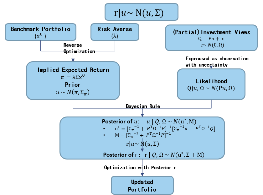
\[\begin{aligned} r|\mu \sim N(\mu, \Sigma) \end{aligned}\]For such an important but ‘dangerous’ exercise on forecasting expected return, we will need to grind every bit of information we have while also account for the significant uncertainty around it.
Aligning this idea, the Black-Litterman (BL) takes investors’ original forecast on expected returns as noisy observations (essentially a partial likelihood) and further anchors it to a robust prior with the Bayes formula. The result is a more informed estimate that emerges as posterior, incorporating both investors’ views and the neutral prior.
The Bayesian Framework within Black-Litterman
One last word before diving into the details. It’s definitely possible to expand the framework to a more general probalistic expressions (I.E. Kolm, Ritter & Simonian (2021) proposed such an expression with much less assumptions that can even incorporate views on hidden factors) while this kind of expansion generally comes with cost of tractbillity and computational burden. Let’s stick to the Gaussian world with the traditional BL models in this blog.
The Prior
The immediate question you might ask (and it is definitely a legit one). You mentioned we are starting from a neutral point in the framework. While you also menteiond the great volatility and ever-changing nature of security return. What should this neutral starting point be? Can we trust any kind of return information to be our neutral start point? Black & litterman’s answer was yes and their choice rest upon the CAPM model.
According to CAPM, market portfolio is the tagent portfolio containing all the information to price expected return of every security (\(E(r) - r_f= r_f + \beta(E(r_M) - r_f)\)). By applying a reversed optimization process, we can effortlessly transform the pricing information embedded in the market weights (\(x_M\)) into its implied return (\(\pi\)).
\[\begin{aligned} max_x & x^T \mu - \dfrac{1}{2}\lambda x^T\Sigma x \\ &\downarrow \\ x_M = (\lambda \Sigma)^{-1} \pi &\leftrightarrow \pi = \lambda \Sigma x_M \end{aligned}\]This implied return is MVO consistent with the market portfolio in the sense that an optimization with it leads exactly to market portfolio. This feature makes the implied return a great neutral point especially when you are benchmarked to the market portfolio. We will stay at the market portfolio until there is a strong enough evidence to deviate.
It is also worth to mention we have other choices of portfolios. Though losing that bit of theoretical support from CAPM, we can switch to other becnmark portfolios for prior extraction. Similarly as the case of the market portfolio, we will get the prior consistent with its corresponding benchmark portfolio. In the financial market where most portfolio managers are benchmarked to some reference portfolios, the technique is of great help.
Formally expressing the prior in mathematics, the prior mean \(\pi\) is set to be the implied return extracted from benchmark portfolio. As for the variance around the prior, a covariance matrix proportional to the return covariance matrix is often employed \(\Sigma_{\pi} = \tau \Sigma\). \(\tau\) is generally set to be \(\dfrac{1}{T}\) or \(\dfrac{1}{T-k}\) making \(\tau \Sigma\) the sampling variance when we are logging the expected return via the security return.
By gathering information from the “conservative” side, we establish a robust starting point in the form of the prior distribution.
\[\begin{aligned} \mu &\sim N(\pi, \Sigma_{\pi}) \\ \end{aligned}\]The Investment View (Likelihood)
With a reasonable and well-founded neutral point established, we can now turn to the more thrilling part of incorporating investment views and forecasts. This is where we unlock the potential for active returns (and for sure perhaps loss). As I see it, this particular aspect of the Black-Litterman model truly embodies its innovation and power.
The BL model handles the investment view as obersavations accompanied by uncentainties (\(\epsilon\)) and further use it as likelihood in a Bayes formula for information combination. Notably, they propose to express all views (absolute or relative) in the form of linear equations with Gaussian noise, enhancing the model’s versatility when dealing with partial views. To capture the uncertainty surrounding these veiws, a diagonal \(\Omega\) is introduced, inversely proportional to investors’ confidence in their respective forecasts (Q). This paradigm allows us to conveniently express our investment views by appropriately modifying the design matrix P.
\[\begin{aligned} Q &= P \mu + \epsilon \\ \epsilon &\sim N(0, \Omega) \\ \Omega &= \begin{pmatrix} \omega_1 & 0 & ... & 0 \\ 0 & \omega_2 & ... & 0 \\ ... & ... & ... & ... \\ 0 & 0 & ... & \omega_k \\ \end{pmatrix} \end{aligned}\]To illustrate this concept further, consider a universe of securities a, b, and c. We can easily establish an absolute view for a subset of this universe—for instance, assuming the expected returns of securities a and b are 5% and 10%, respectively:
\[\begin{aligned} \begin{pmatrix} 0.05 \\ 0.1 \end{pmatrix} &= \begin{pmatrix} 1 & 0\\ 0 & 1 \end{pmatrix} \begin{pmatrix} \mu_1 \\ \mu_2 \end{pmatrix} + \begin{pmatrix} \epsilon_1 \\ \epsilon_2 \end{pmatrix} \end{aligned}\]It is also quite easy and intuitive to incorporate a bunch of relative forecast (such as average expected return of a and b is around c’s and a’s expected return shold be lower than b’s)
\[\begin{aligned} \begin{pmatrix} 0 \\ 0.05 \end{pmatrix} &= \begin{pmatrix} 0.5 & 0.5 & -1\\ -1 & 1 & 0 \end{pmatrix} \begin{pmatrix} \mu_1 \\ \mu_2 \\ \mu_3 \end{pmatrix} + \begin{pmatrix} \epsilon_1 \\ \epsilon_2 \\ \epsilon_3 \end{pmatrix} \end{aligned}\]Since \(\mu\) and \(\Omega\) are the only two source of randomness in the equation. Conditioning on \(\mu\) allows us to derive a partial likelihood in terms of Q, as demonstrated below:
\[\begin{aligned} Q|\mu &\sim N(P\mu, \Omega) \end{aligned}\]This represents our valuable information on expected returns from the “adventurous” side of the equation, guiding us to take bearable and rewardable risk.
The Posterior
Posterior for \(\mu\)
With both prior (\(\mu\)) and likelihood (\(Q\|\mu\)) at our disposal, we are on the verge of obtaining a more refined estimate of the posterior mean.
\[\begin{aligned} \mu &\propto exp((\mu - \pi)^T \Sigma_{\pi}^{-1} (\mu - \pi)) \\ Q|\mu, \Omega &\propto exp((Q - P\mu)^T \Omega^{-1} (Q - P\mu)) \\ \end{aligned}\]It takes the standard Bayes formular along side a few more lines of algebra to derive the posterior for the mean return \(\mu\|Q\).
\[\begin{aligned} \mu|Q, \Omega &\propto \mu * Q|\mu, \Omega \\ \mu|Q, \Omega &\propto exp((\mu - \pi)^T \Sigma_{\pi}^{-1} (\mu - \pi)) * exp((Q - P\mu)^T \Omega^{-1} (Q - P\mu)) \\ &\propto exp((\mu - \mu^{\star}) ^T M^{-1}(\mu - \mu^{\star})) \\ \mu^{\star} &= ((\Sigma_{\pi})^{-1} + P^T\Omega^{-1}P)^{-1}((\Sigma_{\pi})^{-1} \pi + P^T\Omega^{-1}Q) \\ M &= ((\Sigma_{\pi})^{-1} + P^T\Omega^{-1}P)^{-1} \\ &\downarrow \\ \mu|Q, \Omega &\sim N(\mu^{\star}, M) \end{aligned}\]Posterior for r
Having obtained the new BL estimate of \(\mu\), we can now revist the return distribution, which is of utmost importance in application.
\[\begin{aligned} r|Q, \Omega &\propto r|\mu * \mu|Q, \Omega\\ &\downarrow \\ r|Q, \Omega &\sim N(\mu^{\star}, \Sigma + M) \\ \end{aligned}\]In comparison to the original \(r\|\mu \sim N(\mu, \Sigma_{\pi})\), we replace the true \(\mu\) with our refined estimation \(\mu^{\star}\). Simultaneously, the variance expands to \(\Sigma + M\) accounting for uncerntainty around our forecast on expected return as well.
Deviate From a Neutral Point!
After all the groundwork laid out, the moment of revelation has arrived. Does our final result align with the concept of deviating from a neutral point based on investment views, as proposed? The clarity we seek will unfold through a few more algebraic steps.
\[\begin{aligned} \mu^{\star} &= \pi + \Sigma_{\pi}P^T(\Omega + P\Sigma_{\pi}P^T)^{-1} (Q-P\pi) \\ \mu^{\star} &= \pi + Mean Adjustment From View \end{aligned}\]The Black-Litterman estimation \(\mu^{\star}\) can be perceived as sum of prior mean return and an adjustment term accounting for investors’ view to active risk-taking. The difference \((Q-P\pi)\) reflects the disparity between investors’ view and prior mean. It is further scaled by a ratio roughly in the form of \(\dfrac{Prior Variance}{Investment View Variance + Prior Variance}\) adjusted to the return space.
Evidently, two factors collaboratively influence the extent of our deviation from prior.In addition to the distinction between the prior mean and the investment view, the comparison between prior variance and investment view variance also play a pivotal part.
In extreme cases where investment view variance is infinite or prior variance is zero, the BL estimation aligns exactly with the prior mean estimation. Starting from this point, as the investment view variance becomes smaller relative to the prior variance, the BL estimation gradually shifts torward to a blend with higher emphasis on investors’ views. This is an estimation uncertainty awared forecast!
Feeding this refined estimation into an unconstraint Mean Variance Optimization also results in a deviation from the benchmark portfolio. The investment views are added on top of the benchmark portfolio.
\[\begin{aligned} x^{\star} &= (\lambda \Sigma)^{-1} \mu^{\star} \\ &= (\lambda \Sigma)^{-1} (\pi + Mean Adjustment From View) \\ &= x_0 + x_{Mean Adjustment From view} \end{aligned}\]The Shrinkage Perspective
Another representation that offers intuitive insights can be derived from the shrinkage perspective. The BL estimation \(\mu^{\star}\) can be decomposed into weighted average of prior mean and the return mean estimation implied from investment views \(P\mu_{view} = Q\). Though \(\mu_{view}\) is not uniquely defined in case of partial investment views (P is not invertible in the case), it does not hinder us from using it for further insights.
As illustrated below, the sum of the two weights equal to an identity matrix (\(W_0 + W_{view} = I\)). The BL estimation lies within the range spanned by the prior mean and the mean forecast derived from investment views. It is a shrinked estimator, which is commonly used statistical technique to trade accuracy with bias.
\[\begin{aligned} \mu^{\star} &= ((\Sigma_{\pi})^{-1} + P^T\Omega^{-1}P)^{-1}((\Sigma_{\pi})^{-1} \pi + P^T\Omega^{-1}Q) \\ &= ((\Sigma_{\pi})^{-1} + P^T\Omega^{-1}P)^{-1}((\Sigma_{\pi})^{-1} \pi + P^T\Omega^{-1}P\mu_{view}) \\ &= W_0 \pi + W_{view} \mu_{view} \\ W_0 &= ((\Sigma_{\pi})^{-1} + P^T\Omega^{-1}P)^{-1} (\Sigma_{\pi})^{-1} \\ W_{view} &= ((\Sigma_{\pi})^{-1} + P^T\Omega^{-1}P)^{-1} P^T\Omega^{-1}P \\ W_0 + W_{view} &= I \end{aligned}\]What is amazing is that such an BL estimation can be obtained from a Weighted Least Square (WLS) regression with variance depiced in noise term. In this context, both prior and investment views are represented as noisy observation. The regression estimator is exactly the BL estimation.
\[\begin{aligned} \begin{pmatrix} \pi \\ Q \end{pmatrix} &= \begin{pmatrix} I\\ P \end{pmatrix}\mu + e \\ e &\thicksim N(0, \begin{pmatrix} \Sigma_{\pi} & 0 \\ 0 & \Omega \end{pmatrix}) \end{aligned}\]Summary
In the blog, we have delved into the Black-Litterman (BL) model from a Bayesian perspective, and I trust you will found it as valuable a tool for expected return estimation as I have.
The BL model stands out for its exceptional ability to address challenges posed by wild estimation errors when forecasting expected returns. By anchoring the estimation to the implied return from a benchmark, it lays the foundation for a sensible and reliable starting point. Indeed, there can hardly be a better neutral point for mean return than the one implied from a benchmark portfolio. After all, most portfolio managers are benchmarked against specific portfolios (even hedge funds often have their benchmarks, which can be cash or even a simple zero portfolio).
Even with this anchoring mechanism, we recognize the importance of assessing the uncertainty surrounding our ivesment views/forecast. Here is where the brilliance of the Bayesian framework within the BL model shines through. It empowers us to rigorously evaluate uncertainty and make informed decisions, leveraging the available information in a risk-aware manner.
Reference
- Black & Litterman (1991): Global Asset Allocation: combining investors views with market equilibrium
- Idzorek (2007): A Step-By-Step Guide to Black-Litterman Model: Incorporating user-specified confidence level
- Kolm & Ritter (2017): On the Bayesian interpretation of Black-Litterman
- Kolm, Ritter & Simonian (2021): Black-Litterman and Beyond: The Bayesian Paradigm in Investment Management
- Walters (2007): The Black-Litterman Model in Detail