The Covid Recession Update!
The “Big Hit”
In a previous blog Nowcasting: The News From Jagged Economic Data, we have explored the impressive capabilities of a dynamic factor model based nowcasting system to process and interpret the irregular flow of macroeconomic data. However, even such powerful models struggle when confronted with a once-in-a-century (if not once-in-a-millennium) crisis - the Covid recession.
The Covid recession is probably unlike any other economic downturn in history. While most recessions are driven by economic cycles or financial uncertainties, the Covid recession was triggered by a global health crisis. Without much alarm, Covid struck at an unprecendented scale. Factories and stores shut down, and the entire economy came to an abrupt halt.
This shock was vividly reflected in macroeconomic data: US GDP dropped by 31.4% in Q2 2020 - the largest drop since World War II. The country lost 20.5 million (13% of total non-farm) non-farm jobs in April 2020, wiping out 9-year of job growth. The ISM manufactory PMI plummeted to 41, far below the contraction threshold of 50. A clear fat-tail event - the kind that would mess up the estimation of a model. Moreover, the sectoral pattern of economic activities was highly unusual. Sectors typically seen as acyclical such as service and consumption experienced larger contraction, employment no longer lags production, unprecedented liquidity injected to the private sector… etc. Traditional models are ill-equiped to handle such an anomaly!
This raises the critical question: how can we adapt our models to handdle such extreme shocks? What’s the way to produce reasonable estimation with crises like Covid in the data? The New York Fed’s update to their nowcasting model offers valuable insights into these challenges.
Initially introduced in April 2016, the New York Fed’s nowcasting model provided weekly nowcast of US GDP. However, the model was suspended in September 2021 due to “unprecedented fluctuations in many input series during the COVID-19 pandemic posed significant challenges to estimating the model”. Two years later, in September 2023, a new, more robust version of the model was released, designed to better handle such extreme period. Time to take a look at the change!
Here Comes the Change
To appreciate the improvements in the updated model, it’s helpful to take a quick review on the original version first.
The original version is based on a fairly standard dynamic factor model. Macroeconomic indicators are modeled with two components: the latent factors \(f_t\) that stands for comovement and the idyosyncratic disturbance \(\epsilon_t\), which reflect individual series-specific noise. Both components follow autoregressive process with invariant Gassuan noise (\(u_t, e_{i,t}\)) for their own evolution. Special restrictions are applied on the loading matrix \(\Lambda\) during estimation to reflect the cross-sectional correlation structure as well as to incporate quarterly data in monthly flow.
\[\begin{aligned} y_t &= \Lambda f_t + \epsilon_t \\ f_t &= A_1 f_{t-1} + ... + A_p f_{t-p} + u_t \\ \epsilon_{i,t} &= \alpha_i \epsilon_{i, t-1} + ... + e_{i,t} \\ u_t &\sim N(0, Q) \\ e_{i, t} &\sim N(0, I) \end{aligned}\]The advantage of such a parsimonious Gaussian linear system is clear: its simplicity minimized estimation uncertainty, and the Gaussian framework kept calculations tractable, ensuring analytical convenience. Given the small T big P data set at hand, it seems to be a pretty reasonable choice - at least at that time.
However, like any model, it does have its own limitation, which became glaringly evident during the Covid recession. The unprecedented scale and unique sectoral patterns of the Covid recession overwhelmed a system built on invariant parameters. Dramatic fluctuations and disparate structure caused distortions across the entire model, influencing how macroeconomic indicators were interpreted and diggested. To make matters worse, the parameters of this model were re-estimated quarterly using a rolling 15-year window of data. The rabit hole is gonna to be there for the next 15 years.
Given this context, it’s not surprising that the New York Fed suspended this first generation of model shortly after Covid-19 hit. A much-needed new version with update followed. It remains a dynamic factor model but incorporates significant structural changes to handle rapidly evolving volatility and shifted sectoral dynamics more effectively.
Stochastic Volatility and outlier adjustment
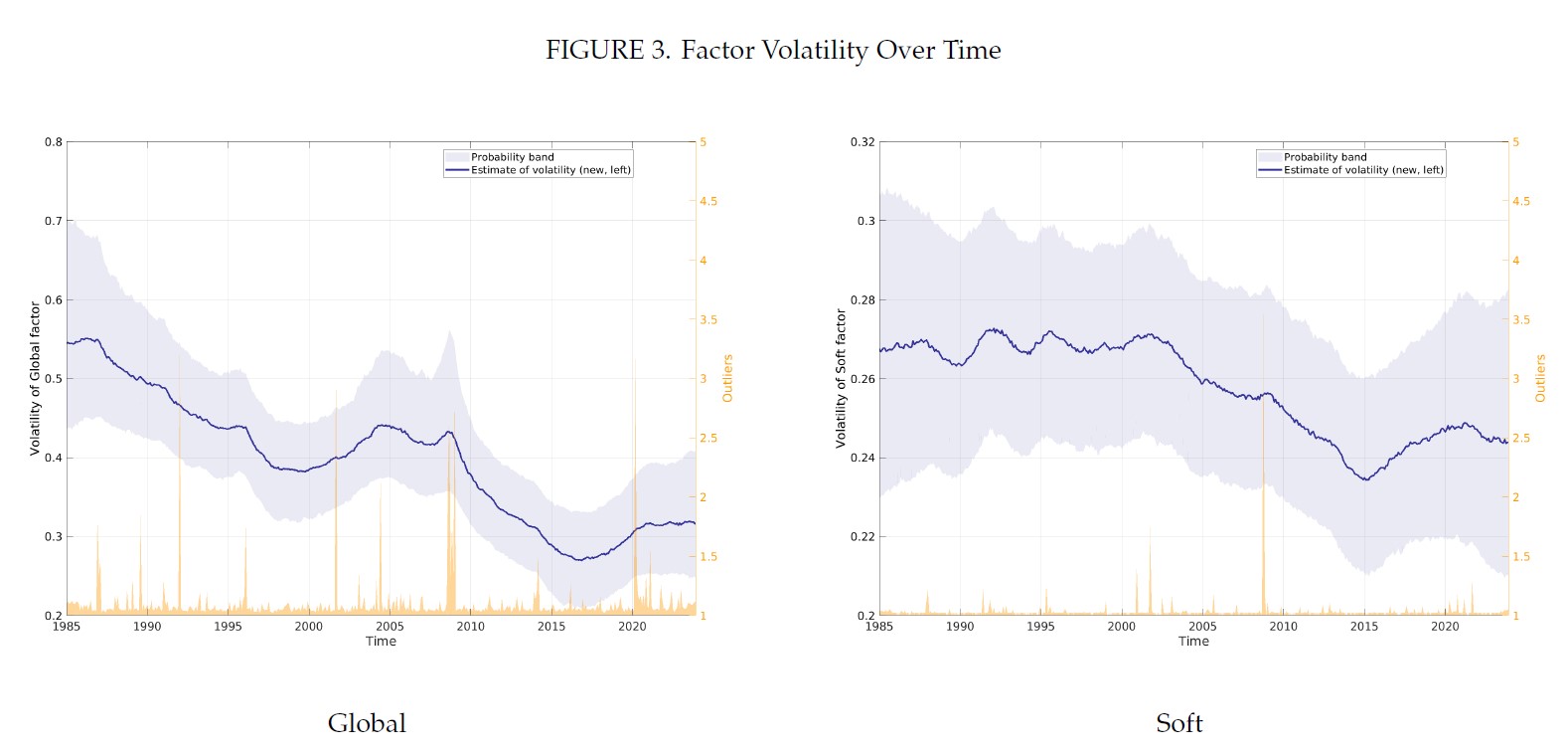
One of the most significant updates to the New York Fed’s nowcasting model is the explicit incorporation of stochastic volatility and outlier adjustments. Rather than relying on Gaussian noise with invariant variance, the updated model introduces the time-varying volatilities (\(\sigma_{ft}, \sigma_{\epsilon t}\)) to account for shifting level of fluctuation. Additionally, discrete outlier multipliers (\(s_{ft}, s_{\epsilon t}\)), which can take values between 1 and 5 are included, allowing for further scalling of fluctuations during extreme events.
\[\begin{aligned} f_t&= A_1 f_{t-1} + ... + A_4 f_{t-4} + \sigma_{ft} \odot s_{ft} \odot e_{ft} \\ \epsilon_t&= \alpha \epsilon_{t-1} + \sigma_{\epsilon t} \odot s_{\epsilon t} \odot e_{\epsilon t}\\ ln \sigma_{ft}^2 &= ln \sigma_{f,t-1}^2 + r_f \odot v_{ft} \\ ln \sigma_{\epsilon t}^2 &= ln \sigma_{\epsilon,t-1}^2 + r_f \odot v_{\epsilon t} \\ v_{ft} &\sim N(0, I) \\ e_{\epsilon t} &\sim N(0, I) \end{aligned}\]This update pushs the model beyond the Gaussian linear realm, but the benefits are substantial. It shields the model from overemphasizing periods of extreme volatility. After all, volatility is the ruler in all estimation and prediction. A distorted volatility estimate due to short-term spikes can disrupt the entire parameter estimation process, leading to skewed forecasts.
By incorporating time-varying volatility and outlier adjustments, the model is better equipped to handle large fluctuations. Sharp, rapid changes—such as those seen during the Covid recession—are now interpreted more locally, reducing the likelihood that these events will distort the broader model or influence forecasts for unrelated periods.
Factor Structure
Another significant change is the inclusion of the “Covid factor” as an additional latent factor to capture the unique economic dynamics of the Covid recession. This factor is active only from March to September 2020, and loads on most economic indicators, with the exception of those inflation ones.
Given the unprecedented nature of the Covid crisis, it’s remarkable (and somewhat surprising) that a single latent factor could adequately capture its effects. While this is indeed the case! Maroz, Stock, and Watson (2021) found that adding a Covid factor significantly improved model fit, boosting the R-squared from 0.23 to as high as 0.8 in their effort to generalize 127 macroeconomic indicators using three latent factors.
Their findings also showed that the Covid factor is most relevant between March and June 2020, phasing out gradually afterward, which generally aligns with the New York Fed’s decision to apply the factor from March to September. In their estimation, the Covid factor demonstrate a sharp economic decline in April, followed by a strong rebound peaking in June.
Interestingly, introducing the Covid factor influenced the behaviors of other latent factors differently. For example, during Covid recession, while extreme fluctuations persisted in the “Global factor” that loads on all macroeconomic indicators, the fluctuations within the “Soft factor” (which primarily loads on survey indicators) is largely absorbed into the Covid factor. This highlights the varied responses of soft indicators like PMI compared to hard data, such as industrial production, during the pandemic.
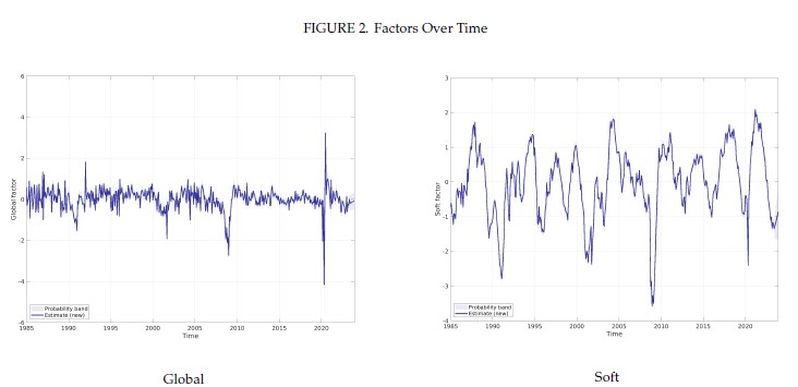
Source: Almuzara, Baker, O’Keeffe & Sbordone (2023): The New York Fed Staff Nowcast 2.0
Additionally, the New York Fed introduced a long-term growth trend factor, which specifically loads on GDP and GDI indicators, to capture shifts in long-term economic growth.
\[\begin{aligned} y_t & = \mu + l g_t + \Lambda f_t + \epsilon_t \\ g_t &= g_{t-1} + r_g v_{gt} \\ v_{gt} & \sim N(0,1) \end{aligned}\]Looking at the long-term growth trend estimated over the past 15 years, the need for this factor may not seem pressing. The estimated long-term growth rate has remained around 2.6%, with a relatively wide 90% probability band, suggesting that even without this factor, the impact on the model would be limited.
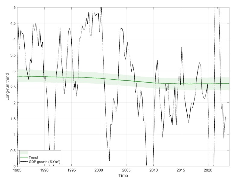
Source: Almuzara, Baker, O’Keeffe & Sbordone (2023): The New York Fed Staff Nowcast 2.0
The real motivation behind adding this factor is likely to improve the model’s robustness so that more data of longer history can be incororated for estimation. With the new structural elements introduced, it’s both logical and necessary to use a broader dataset. On one hand, the model is now better equipped to handle periods of high fluctuation, like the Covid recession in the history. On the other, the increased complexity—especially the significantly increased number of parameter and the introduction of nonlinearity—demands a larger dataset for reliable estimation.
And using more data is precisely what the New York Fed did with their model update. Instead of relying on a rolling 15-year window for estimation, they now use the entire sample. As the dataset expands over time, the need to account for changing long-term growth rates becomes more relevant.
And More
With the significantly updated nowcasting system incorporating more sophisticated structures, improved GDP nowcasts during the Covid recession were achieved as expected. However, these improvements came at a cost. The relatively lightweight Expectation Maximization (EM) algorithm that worked for the earlier, simpler models proved inadequate in handling the increased complexity and nonlinearity of the new system.
To address this, the authors switched to a Gibbs sampler—a multi-dimensional version of Monte Carlo Markov Chain (MCMC) simulation—to derive posterior distributions. In response to the rising complexity, each parameter in the model is assigned a prior distribution, and a long sequence of Markov Chain iterations is ran until convergence. Each iteration involves 10 steps of sequential parameter draws, making this process intensive and challenging both in terms of implemetation and computational time.
The shift to Bayesian estimation using Gibbs sampling offers benefits as well. Rather than the solely point estimates from the EM algorithm, the new approach provides full posterior distributions for each parameter, enabling deeper insights. For instance, the volatility of latent factors can now be directly inferred from these posterior distributions. This expanded information, however, comes with a tradeoff — more data is required.
Looking back, the previous nowcasting system, with its invariant parameters and reliance on a rolling window of data, assumed that market conditions would remain relatively stable over short periods. The Covid recession, with its swift and unprecedented economic impact, shattered this assumption. To cope with the rapidly changing market, dynamic elements like time-varying volatility and long-term growth trends were introduced, further increasing the demand for more data.
Given the growing geopolitical tensions, re-organized supply chain, and slowing global growth, it wouldn’t be surprising to see further and more frequent structural shifts in the market, necessitating even more complex models. As we move forward, we are more and more in the situation to decide the complexity of a model, which is required to adapt to a changing market and bounded by the availability of data. The key, as implied in New York Fed’s model update, is probably in making smart decisions about where and how to introduce this complexity without overburdening the model or losing sight of data constraints.
Reference
- Almuzara, Baker, O’Keeffe & Sbordone (2023): The New York Fed Staff Nowcast 2.0
- Almuzara, Baker, O’Keeffe & Sbordone (2023): Reintroducing the New York Fed Staff Nowcast
- Bok, Caratelli, Giannone, Sbordone & Tambalotti (2017): Macroeconomic Nowcasting and Forecasting with Big Data
- Maroz, Stock & Watson(2021): Comovement of Economic Activity During the Covid Recession
- Antolin-Diaz, Drechsel & Petrella (2023): Advances in Nowcasting Economic Activity: The Role of Heterogeneous Dynamics and Fat Tails