A First Glimpse into the “Factor Zoo”
The Factor Zoo
In our previous blog, The Adjustment for Luck, we embarked on an exploration of how to identify factors that genuinely drive cross-sectional security returns out-of-sample in the real world. We focused on one critical challenge in this journey: the multiple testing problem. Essentially, when factors are identified through extensive searches, their apparent in-sample predictive power often owes more to luck than to true predictive ability. The massive number of factors published, not to mention the countless others tested behind the scenes, highlights just how exhaustive researchers have been in this quest. In the face of this typical multiple testing scenario, the traditional 1.96 t-statistic threshold no longer ensures a 5% Type I error rate.
The bootstrap method also discussed in that blog comes as an attempt to mitigate this problem. By combining a customized orthogonalization technique, which sets up a purified null hypothesis that holds by design, with bootstrapping, researchers can establish more reliable baselines for statistical tests. While it’s not a perfect solution - we are still subject to a sample of smaller size compared to number of factors with evolving distribution, it’s certainly a solid starting point.
It’s time to continue our exploration! With hundreds or even thousands of factors (what Cochrane called the ‘Factor Zoo’ in his presidential address to the American Finance Association), there is plenty more observations, challenges and models to discuss!
Looking a bit closer at this massive collection of factors, each claiming to predict cross sectional security returns, we notice it doesn’t quite align with the conventional wisdom in the investment community: predicting expected returns is really difficult. If these documented factors truly possessed even modest predictive power marginally, we’d be well-equipped to forecast returns by combining them. Yet, that’s not the case. Something seems off about this ‘Factor Zoo’, and it’s definitely worth digging into.
So, what can we take from the Factor Zoo? How should we interpret it? In this blog, let’s start this quest by examining two opposing views on the matter.
The Skeptical and The Optimistic
First, let’s consider the perspective offered by Hou, Xue, and Zhang (2020). In their paper ‘Replicating Anomalies’, they shed light on the Factor Zoo by undertaking an ambitious task of replicating nearly 200 published factors. Using a comprehensive dataset of the U.S. stock market spanning from 1967 to 2016, they evaludated each factor’s predictive power under the same test procedures of sorted long-short portfolios across three investment horizons (1, 6, and 12 months). The findings were sobering: 65% of the factors failed to surpass the traditional t-statistic threshold of 1.96. When a stricter threshold of 2.78 was applied to account for multiple testing corrections, the failure rate climbed further to an astonishing 82%!
Why such dismal replication rates? The authors believe one of the key driver is the excessive emphasis on illiquid micro-cap stocks in earlier factor research. Many factors show much stronger predictive power among smaller stocks,likely due to the lower levels of investor attention they recevie and higher transaction costs required to arbitrage them. These micro-cap stocks can account for as much as 60% of the total number of stocks but as little as 3% of the total market capitalization, representing investment opportunities with questionable capacity and profitability. Weighting these micro-cap stocks equally as the other 97% in factor portfolio construction or regression as some previous factor research did creates a significant imbalance and skews the conclusions more favorably toward significance.
Another equally important driver contributing to the low replication rate lies in the dataset used. Hou, Xue, and Zhang utilized a 50-year dataset of U.S. security returns, which is much more comprehensive than the datasets employed in many earlier factor studies. In the financial market with an inherently low signal-to-noise ratio, it’s not surprising for a factor to perform well in localized samples but falter in broader datasets. This is especially true when there’s an incentive to customize the sample to achieve greater significance for publication.
There’s also a much more optimistic angle to this discussion. In their article “Is There a Replication Crisis in Finance”, Jensen, Kelly, and Pedersen (2023) offered a contrasting perspective. Utilizing an even broader dataset spanning 93 countries and applying their innovative Bayesian testing framework, they reached a significantly different result: an 82% replication success rate.
82% vs 35%! How could the outcomes diverge so dramatically? Jensen et al. delved into this intriguing discrepancy themselves. As summarized in the chart below, several differences in test procedure and datasets are behind this divergence in replication rates.
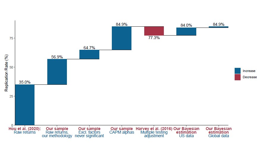 Source: Jensen, Kelly & Pedersen (2023): Is There a Replication Crisis in Finance
First and perhaps most importantly, the construction of factor returns differs significantly between the two studies. Instead of using the raw returns of the long-short factor portfolios, as Hou et al. did, Jensen et al. opted to use the CAPM alpha, which is essentially the regression residual of the raw factor return over market portfolio. This change alone increased the successful rate by over 20%!
Removing exposure to market beta definitely has its merits. After all, we are aiming to identify factors that can provide additional predictive power in addition to traditional ones like market beta. However, it’s important to note that this approach might introduce some unintended distortions. For instance, when testing the low volatility factor, the original intend is to evaluate whether stocks with lower volatility outperform the others. While when regressing out the market return to the CAPM alpha, it actually turns the low volatility factor into something similar to the betting against beta factor - a distinct factor. We might be testing something different than we initially thought.
The remainder of the replication rate increase can be traced to various, somewhat less influential adjustments in test procedures and datasets. For instance, Jensen et al. opted to cap market value weights in their factor portfolios to prevent mega-cap stocks from exerting an outsized influence. They also focused exclusively on a 1-month holding period and utilized a longer dataset. While these changes might seem minor, they collectively contributed to the improved replication outcomes.
The Take
Now that we’ve acknowledged the existence of the Factor Zoo, it’s evident that our impressions of these factors can vary widely, depending on the test procedures used and the datasets examined. The methods researchers choose to construct and evaluate factors can lead to strikingly different conclusions about their predictive power and reliability. So, what can we learn from all this complexity?
From an investor’s point of view, constructing portfolios and, by extension, designing the testing procedures is far from a one-size-fits-all endeavor. It heavily depends on the investor’s unique profile, the range of investment opportunities available, and their sensitivity to practical constraints like evaluation horizons and transaction costs. As a result, investors may employ widely different methods to gain factor exposures in portfolio construction, ultimately leading to a broad spectrum of performance outcomes.
For example, an asset owner focused on long-term strategic allocation might find Jensen et al.’s exclusive use of a one-month horizon less meaningful. Conversely, a hedge fund pursuing arbitrage with efficient trade execution might consider Hou et al.’s market-value weighting scheme too restrictive. From this perspective, there’s no absolute right or wrong — different testing approaches resonate with different investors. The key is to understand how testing decisions influence results and ensure they align with the realities of portfolio construction in real world.
However, this doesn’t mean that investors operating under similar portforlio construction procedures to Jensen et al. should celebrate the 82% replication rate as a guaranteed path to accurate forecasts. Even with this encouraging number, they can’t simply combine hundreds of “working” factors and expect to produce a significantly improved prediction of future returns. Many factors share similar ground in explaining returns, so adding highly correlated factors offers little to no extra predictive power. Acknowledging this, Jensen et al. used a hierarchical Bayesian model, organizing all the factors into 13 categories, within each factors often displayed strong correlations.
It becomes even trickier when we consider the differences in datasets used for testing. While a larger dataset might inspire greater confidence hence the dataset used in Jensen et al.’s research might be preferred for its longer history and wider coverage. This advantage hinges on the assumption that distributions remain consistent across both time and geography. Unfortunately, this isn’t always the case. Market movements from 70 years ago, during World War II, may offer little insight into contemporary investment strategies. Likewise, it’s hardly surprising that financial markets around the world operate under diverse structures, further complicating the hope of universal applicability with an unconditional model.
And yet, the list of challenges don’t end there. Even if we manage to find a robust dataset and employ appropriate testing procedures closely aligned with real-world investing (which is already quite difficult due to the limited data available acompanied by ever-chaging market), will these results still hold true tomorrow?
How do we translate yesterday’s insights into tomorrow’s actions? How can we navigate from insights drawn from dataset in the past to actions in the future? This might be the biggest puzzle in forecasting security returns. In truth, there may never be a perfect or even a good enough method to bridge this gap. Investors typically rely on the fact that markets, while volatile, rarely pivot 180 degrees overnight, allowing us to glean useful information from the recent past. This is also where structural models can shine. By providing a framework with clearly defined assumptions and logical connections, these models can guide us more reliably than raw empirical results alone, helping us understand what’s happening and what might come next.
Reference
- Jensen, Kelly & Pedersen (2023): Is There a Replication Crisis in Finance
- Hou, Xue & Zhang (2018): Replicating Anomalies
- Cohcrane (2011): Discount Rates