Holding Discipline for Drawdown Control
Introduction
In a previous blog From Volatility to Maximum Drawdown, we delved into the widely quoted risk measure, maximum drawdown, exploring factors impacting it and uncovering pain points in its analysis and control. Following on the discussion, it’s time to explore practical approaches to integrate drawdown management into a portfolio management process explicitly.
The landscape of drawdown control is undeniably shaped by critical judgments made at pivotal moments of market fluctuations and regime shifts. Often, a well-founded judgement regarding the efficacy of a strategy, even executed with basic rules in holding discipline, can shield investors reasonably from intolerable drawdowns.
While the explicit integration of drawdown control offers additional advantages, especially within a systematic portfolio management framework. To start, it assists in conveying a consistent portfolio language, facilitating both ex-ante ex-post attribution — crucial components for informed decision-making and continuous improvement. Moreover, in scenarios where confident judgment is unattainable, the explicit inclusion enables us to bridge the gap with backup plans rooted in clearly defined assumptions.
With these benefits in mind, our focus in this blog turns to a journey of tool excavation, catering around the risky asset holding discipline pioneered by Grossman & Zhou (1993). This discipline advocates for investing a constant proportion of the largest acceptable loss in risky assets to maximize expected utility growth within the desired drawdown range. The optimal holding derived from this approach can serve as a reference for leverage of the risky asset mix, whether on a regular basis or in response to significant deviations.
Optimal Holding with Drawdown Control
Let’s begin by taking a closer look at the holding discipline.
Assume \(W_t\) represents the value of wealth at time t and \(M_t\) denotes the highest wealth level achieved before or at t. To manage drawdown, Grossman & Zhou (1993) introduced a hard constraint on maximum drawdown, which is formulated as a stochastic floor determined from previous peak value (\(W_t \geq \alpha \mathop{Max}_{0\leq s\leq t}{W_s}\), \(1 - \alpha\) is the maximum acceptable drawdown). This constraint is imposed upon the classical portfolio optimization problem of maximizing the long term expected growth of power utility (\(U(W) = \dfrac{W^{1-A}}{1-A}\)).
Accounting for different time values of current wealth and previous peak, we are essentially conducting the following portfolio optimization. (\(X_t\) is the amount of money invested in the risky asset).
\[\begin{aligned} \mathop{Max}_{X_t} & \mathop{lim}_{T\to \infty} \dfrac{1}{(1-A)T}lnE[(1-A)U(W_T)] \\ & P[W_t \geq \alpha e^{rt}\mathop{Max}_{0\leq s\leq t}(W^{\pi}_s e^{-rs}), 0\leq t\leq \infty] = 1 \end{aligned}\]This portfolio optimization problem, with its time dynamics, probabilistic expressions, and expectations, is undoubtedly challenging. Fortunately, we stand on the shoulders of the giants :). Grossman & Zhou (1993) and Cvitanic & Karatzas (1994) solved the problem and derived the optiomal holding in risky asset analytically.
\[\begin{aligned} X_t &= \dfrac{\mu}{\sigma^2} \dfrac{1}{(1 - \alpha)A + \alpha} (W_t - \alpha M_t) \\ &= \dfrac{\mu}{\sigma^2} \dfrac{1}{(1 - \alpha)A + \alpha} (1 - \alpha\dfrac{M_t}{W_t})W_t \\ M_t & = e^{rt}\mathop{Max}_{0\leq s\leq t}(W^{\pi}_s e^{-rs}) \end{aligned}\]Despite the lenghty derivation, the optimal holding derived is quite intuitive, resembling the Constant Proportion Portfolio Insurance(CPPI) type. By investing a constant proportion \(\dfrac{\mu}{\sigma^2} \dfrac{1}{(1 - \alpha)A + \alpha}\) of the the maximum acceptable loss (difference between current wealth and lowest acceptable wealth level defined by prior peak \(W_t - \alpha M_t\)) in the risky assets, we can maximize expected power utility growth while restricting maximum drawdown below (\(1 - \alpha\)) almost surely.
Obviously, this downside protection comes at the cost of a lower rate of wealth accumulation. As we raise the maximum drawdown threshold from 0 to \(1 - \alpha\), the expected log utility growth is scaled by \(1 - (1 + \dfrac{1-\alpha}{\alpha}A)^{-1}\)
This holding aligns with our intuitive understanding of relevant factors in drawdown control: a larger ‘safe cushion’ above the threshold (\(W_t - \alpha M_t\)), enhanced expected performance of the risky asset (\(\dfrac{\mu}{\sigma^2}\)), lower risk aversion (A) and a higher acceptable maximum drawdown level (\(1 - \alpha\)) justify for a more substantial allocation to the risky asset. It’s crucial to note that the optimality of this risky asset holding persists even in the case of deterministic changing parameters of \(\mu\) and \(\sigma\). In such cases, the proportion would dynamically adjust with changes in \(\mu\) and \(\sigma\) changes, allowing for much more flexible applications.
Two Handy Variants
This optimal holding can be further tailored to suit various other use cases in drawdown management.
Firstly, it can be extended to the scenario of drawdown defined by an absolute amount of wealth. In situations where investors aim to retain at least K dolloars instead of some percentage of the previous peak, the optimal holding can be modified slightly to account for the change. Essentially it is equivalent to replace the constraint on floor from the stochastic \(M_t\) to a constant K, leading to the safe cusion change from \(W_t - \alpha M_t\) to \(W_t - K\) and risk aversion adjustment from \((1 - \alpha)A + \alpha\) to \(A\).
\[\begin{aligned} Y_t &= \dfrac{\mu}{\sigma^2} \dfrac{1}{A} (W_t - K) \\ \end{aligned}\]Additionally, it can also be extended to a scenario with multiple risky assets, as explored by Cvitanic & Karatzas (1994). Such expansion provides the flexibility to choose the granularity of risky asset classification. For example, one can allocate funds within equities and treasury bond or more specifically within large-cap equity, small-cap equity, government bonds, credit bonds, and money market instruments - all under the same framework with a constraint on drawdown. Such flexibility would be quite helpful especially when our judgment may cover partially on the investment universe
\[\begin{aligned} X_t = \mu {(\sigma^{-1})}^2 \dfrac{1}{(1 - \alpha)A} (W_t - \alpha M_t) 1 \\ \end{aligned}\]The practical Side
Now equipped with a clearly defined optimal holding in the risky asset, continuous re-allocation to these assets/portfolios as per the derived optimal holding, paves the way for maximized wealth utility growth within a predefined drawdown level almost surely!
\[\begin{aligned} X_t &= \dfrac{\mu}{\sigma^2} \dfrac{1}{(1 - \alpha)A + \alpha} (W_t - \alpha M_t) \\ Y_t &= \dfrac{\mu}{\sigma^2} \dfrac{1}{A} (W_t - K) \\ \end{aligned}\]This optimal holding naturally fits into a two-step portfolio construction process. The initial step involves building portfolios of risky assets, followed by determining the allocation within these portfolios and the risk-free asset based on the optimal holding derived. This two-step process can be applied regularly during each rebalancing, in response to significant deviations from the optimal risky holding, or in both scenarios.
The immediate question arises: how frequently should we rebalance, and what magnitude of deviation warrants a response? This tradeoff involves considerations of tolerances on breaking the maximum drawdown threshold, transaction costs, and return. On one side, the optimality of the risky asset holding is rooted in continuous allocation. More frequent rebalancing and responding to smaller deviations increase the likelihood of meeting the maximum drawdown threshold. As a cost, they result in higher transaction costs and lower holdings in the risky asset, leading to a potential loss in expected returns.
To aid in decision-making on this tradeoff, insights from the perspective of contingent claims can be valuable. One may already notice the similarities and links between this dynamic holding on risky asset and an option instrument on the same. It turns out that, entering into a call option with payoff of loss excessive of the maximum drawdown threshold (\(max(realized MDD - MDD threshold, 0)\)) provides similar protection against a predefined maximum drawdown threshold, albeit without considering the reward side. Such a contigent claim is an exotic option with abundant analytical tools available out there.
For instance, Vercer (2006) conducted simulations on the delta exposure of this option across various maximum drawdown (MDD) and current realized drawdown (drawdown) scenarios. Considering that a delta hedging portfolio of underlying can replicate this option that provides drawdown protection, delta is actually an indicator of risk exposure to maximum drawdown - independent of risk aversions and estimations of expected returns.
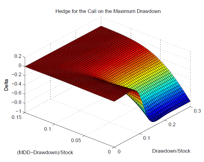
source: Vecer (2006): Maximum Drawdown and Directional Trading
Insights from the perspective of contingent claims extend beyond the delta plot. Meaningful insights can be gained from Gamma, the derivative of delta as well. Higher gamma indicates volatile exposures to delta, suggesting the need for more frequent rebalancing and a lower deviation range for the quickly changing exposure. Similar Monte Carlo simulations can help evaluate exposures to maximum drawdown in the form of delta and other Greeks under different circumstances of volatility, drift, big jumps, and more. The numerous tools in the arsenal of derivative analysis can provide a wealth of insights in addition to an optimized portfolio.
Lastly, but certainly not least, it’s also worth examining the parameters required for the calculation of this optimal holding. Among the components of the optimal holding, the drawdown threshold is predefined, and the current drawdown is readily observable. Regarding risk aversions, expected return, and volatility, they are standard inputs to a traditional Markowitz portfolio optimization. Adding drawdown protection to a Markowitz-based portfolio management process without requiring additional estimation tasks is plausible.
Opting for the same parameters in both steps of the portfolio construction process is a valid choice. However, there are cases where it may not be desirable or even possible to do so. For the latter, numerous risk-centric portfolio construction models as we discussed in the “The Conviction Pyramid of Portfolio Construction” are employed to avoid estimating expected return due to its instability. For the former, there is indeed a reason to use different sources of estimation. Estimation errors themselves can contribute to drawdown, making it reasonable, from a risk management perspective, to derive parameters for drawdown control from diverse sources. In either scenario, we retain the flexibility to articulate explicit and clearly stated assumptions concerning expected return, volatility, or Sharpe ratio, aligning them with the specific nuances of the case at hand.
Reference
- Grossman & Zhou (1993): Optimal Investment Strategies For Controlling Drawdowns
- Cvitanic & Karatzas (1994): On Portfolio Optimization Under “Drawdown” Constraints
- Vecer (2006): Maximum Drawdown and Directional Trading
- Busseti, Ryu & Boyd (2016): Risk-Constrained Kelly Gambling