Oh, VIX!
- Introduction
- Expected Volatility under Q
- The anticipated volatility and the market take
- Appendix
- Reference
Introduction
There is the subtle feeling when reading into a ‘small’ yet delicate modeling like volatility index (VIX) at an era of roaring LLMs! Like many, I found myself astonished by the insights, judgement and beyond that can be gained from LLM via matrix operations involving hundreds of billions of parameters.This marvel doesn’t diminish my admiration for the thought and inspiration behind a refined structural model like the VIX. Still interesting to read into it :)
This exploration originally stemmed from a dive into portfolio drawdown control. In the previous blogs From Volatility to Maximum Drawdown and Holding Discipline for Drawdown Control, we dissected the impact of pivotal factors on the risk measure of maximum drawdown and strategies for its control within an (unconditional) stochastic return process. Clearly, the vast expanse of market data offers boundless possibilities, one of which is the VIX. As a market anticipation of future realized volatility, it naturally links to risk regimes and, subsequently, the performance of risky assets.
In this blog, let’s delve into the beauty of the VIX, exploring its intuition and embedded information. A quick spoil alert on everything we are gonna to discuss - The VIX represents the market’s anticipation of future realized volatility, explicitly defined through a hypothetical variance swap and valued by the weighted average price of options spanning a wide range of strike prices.
Expected Volatility under Q
Why bother to construct an index from options rather than examining individual options themselves? While it’s true that an option’s premium reflects views on future volatility of the underlying asset, its sensitivity to volatility (vega) constantly fluctuates based on the option’s moneyness, leading to a somewhat blurred picture. What we aim for is a more focused instrument with consistent volatility exposure.
Back in 1999, Demeterfi, Derman, Kamal & Zou (1999) provided one such solution in a sell side research report, laying the groundwork for what would become the now-famous CBOE VIX index. The essence lies in pricing a variance swap with payoff (V - K), where V is the future realized volatility (\(V = \frac{1}{T}\int_o^T\sigma^2(t,...)dt\)) and K is the predefined delivery price.
To value this variance swap, we employ a common strategy used for most derivatives: taking the expectation of its payoff under the risk-neutral probability measure: \(F = E^Q[e^{-rT}(V - K)]\). the fair delivery price should equal the expectation of future realized volatility under the risk neutral measure - a price that mirrors future volatility and serves as a natural measure for it:
\[\begin{aligned} K_{var} &= E^Q[V] \\ &=\frac{1}{T}E^Q[\int_o^T\sigma^2(t,...)dt] \end{aligned}\]Unfortunately, the instantaneous variance (\(\sigma^2(t,...)\)) remains unknown, we can not calculate \(K_{var}\) directly with the formula. Following the spirit of relative pricing with dynamic replication, it turns out that a well designed portfolio of options (and futures) on the underlying will do us the favor for pricing \(K_{var}\).
To simplify, through mathematical derivations (detailed in the appendix), we initially construct a portfolio consisting of a dynamic underlying and a static hypothetical log contract. Eventually, this evolves into a portfolio of options weighted in proportion to the inverse of their strike price squared. Here, \(S_{\star}\) is an arbitrary price, facilitating numerical calculations, with the first few terms beyond the option price serving as adjustments for this flexibility.
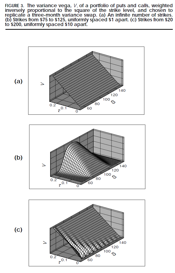
\[\begin{aligned} K_{var} &= \frac{2}{T}[rT - (\frac{S_0}{S_{\star}}e^{rT} - 1) - log\frac{S_{\star}}{S_0} \\ & + e^{rT}\int_0^{S_{\star}} \frac{1}{K^2}P(K)dK \\ & + e^{rT}\int_{S_{\star}}^{\infty} \frac{1}{K^2}C(K)dK ]\\ \end{aligned}\]It’s much easier to verify that such a portfolio of options scaled by \(\dfrac{1}{K^2}\) has a constant vega under the assumption of BSM (Black-Schole-Schole option pricing). To make the portfolio vega invariant to underlying price, set the partial derivative to 0 leads to the weight proportional to \(\dfrac{1}{K^2}\). It should be noted that this property, as well as the calculation of VIX, do not rely on BSM assumptions.
\[\begin{aligned} vega &= \frac{\partial C}{\partial \sigma^2} = \frac{S\sqrt{\tau}}{2\sigma}\frac{exp(-d_1^2/2)}{\sqrt{2}\pi}\\ \Pi &= \int_{0}^{\infty} w(k) O(S, K, v) dK \\ vega_{\pi} &= \int_{0}^{\infty} w(k) vega_o(S,K,v) dK \\ \end{aligned}\] \[\begin{aligned} \frac{\partial vega_{\Pi}}{\partial S} &= 0 \\ \downarrow \\ 2w(k) + K\frac{\partial w(k)}{\partial K} &= 0 \\ \downarrow \\ w(k) &= \frac{const}{K^2} \end{aligned}\]This concept is also exemplified in the simulation of Figure 3a from DDKZ(1999), where a portfolio with an infinite number of options, appropriately weighted by different strikes, retains invariant vega regardless of underlying asset price movements or the passage of time, effectively replicating the variance swap.
Source: DDKZ(1999): More Than You Ever Wanted to Know About Volatility Swaps
The anticipated volatility and the market take
Now armed with a portfolio of tradable options with observed prices to replicate the hypothetical variance swap, we can discern how this calculation encapsulates vital information about the full distribution through its utilization of options with varying strikes. But what economic insights does it unveil?
Understanding that the price of a derivate is essentially its discounted expected payoff under risk neutral probability in a complete market without arbitrage opportunity, we recognize the VIX as the price of a derivative that pays future realized volatility, adjusted for time value. Consequently, market views of heightened future volatility and increased risk aversion drive up the price of this derivative, thus elevating the VIX.
\[\begin{aligned} VIX = K_{var}&=\frac{1}{T}E^Q[\int_o^T\sigma^2(t,...)dt] \\ &= E^Q[V] \\ &= e^{rT}P(V) \end{aligned}\]This is aligned with empirical research. Jiang & Tian (2005) identified the SPX VIX as a reliable estimator of future realized volatility, even when controlled for other indicators such as historical realized volatility. Their regression analysis revealed that while the slope on historical volatility loses significance, the slope on VIX remains significant, underscoring VIX’s efficacy as an improved estimator of future volatility to a certain extent.
Moreover, what makes the VIX even more intriguing is its tendency to be larger than the future realized volatility of the corresponding period, indicating investors’ attitude towards future risk. Carr & Wu (2008) exploited this disparity to measure the variance risk premium, asserting that “investors are willing to pay extra money to enter into variance swap because they dislike variance, not just because it is anti-correlated with stock prices, but on its own right.” This perspective has led many to contemplate variance as an asset class in its own right.
Undoubtedly, both the magnitude of volatility and the market’s sentiment towards risk significantly impact the performance of risky assets and, consequently, considerations in portfolio management. For instance, the SPX VIX often exhibits concurrent or even leading peaks during times of significant turmoil in the US equity market. Thus, whether analyzing the VIX’s time dynamics on its own or alongside further calibrated indicators such as its term structure or deviation from recent realized volatility, it proves to be a valuable tool deserving of attention when managing a portfolio.
Appendix
\[\begin{aligned} K_{var} &= \frac{1}{T}E^Q[\int_o^T\sigma^2(t,...)dt] \\ &= \frac{2}{T} E^Q[\int_0^T \frac{dS_t}{S_t} - d(logS_t)] \\ & = \frac{2}{T} E^Q[\int_0^T\frac{dS_t}{S_t} - log(\frac{S_T}{S_0})] \end{aligned}\]It is clear that, exposue to variance can be obtained via 2 positions:
- a dynamic position on \(\frac{1}{S_t}\) share of the underlying
- a static position on log contract
Based on the assumption, we can get the expectation of part 1 as \(E^Q[\int_0^T \frac{dS_t}{S_t}] = rT\)
As to part 2 (the static log contract), we can obtain the log contract via the portfolio of forward and options.
\[\begin{aligned} log \frac{S_T}{S_0} &= log\frac{S_T}{S_{\star}} + log\frac{S_{\star}}{S_0} \\ -{log\frac{S_T}{S_{\star}}} & = -\frac{S_T - S_{\star}}{S_{\star}} \\ &+\int_0^{S_\star} \frac{1}{k^2} Max(K-S_T, 0)dK \\ &+\int_{S_\star}^{\infty} \frac{1}{k^2} Max(S_T - K, 0)dK \end{aligned}\]- A short position in \(\frac{1}{S_{\star}}\) forward contracts struk at \(S_{\star}\)
- A long position in \(\frac{1}{K^2}\) put options struck at K for all strikes from 0 to \(S_{\star}\)
- a similar long position in \(\frac{1}{K^2}\) call options struck at K, for all strikes from \(S_{\star}\) to inf.
Take the expectation of the 2 position we got so far. We can get the VIX as below. It should be noted that \(S_{\star}\) is an arbitrary number.
\[\begin{aligned} K_{var} &= \frac{2}{T}[rT - (\frac{S_0}{S_{\star}}e^{rT} - 1) - log\frac{S_{\star}}{S_0} \\ & + e^{rT}\int_0^{S_{\star}} \frac{1}{K^2}P(K)dK \\ & + e^{rT}\int_{S_{\star}}^{\infty} \frac{1}{K^2}C(K)dK ] \end{aligned}\]Reference
- DDKZ(1999): More Than You Ever Wanted to Know About Volatility Swaps
- CBOE vix white paper
- Jiang & Tian (2005): The Model-Free Implied Volatility and Its Information Cotent
- Jiang & Tian (2009): Extracting Model-Free Volatility from Option Prices: An Examination of the VIX Index
- Carr & Wu (2008): Variance Risk Premium